
Maxwell’s Unification of Electricity and Magnetism Explained
Understand how changing electric and magnetic fields are linked, why Maxwell added displacement current, and how this leads to electromagnetic waves. Includes worked examples and challenging HSC-style questions.
Sunlight can cross about 150 million kilometres of near-vacuum to reach Earth. Sound cannot do that: without matter to vibrate, a sound wave has nowhere to go. So if light is a wave, what exactly is oscillating?
That question becomes much more interesting once you remember two earlier discoveries. A changing magnetic field can produce an electric effect. An electric current can produce a magnetic field. Maxwell’s crucial step was to complete the connection: a changing electric field also contributes to a magnetic field.
Before going further, make a prediction. If a magnetic field changes and can produce an electric field, what would make the theory more symmetrical: should a changing electric field also produce a magnetic effect?
Yes. That missing link is what turns electricity and magnetism from two related topics into one theory of electromagnetism – and allows the theory to predict travelling electromagnetic waves.
01Start with the simpler field picture
An electric field tells you what force a charge would experience at a point in space. For a charge \(q\) in an electric field of magnitude \(E\),
\[
F_E=qE
\]
where \(F_E\) is the electric force in newtons (N), \(q\) is charge in coulombs (C), and \(E\) is electric field strength in newtons per coulomb (\(\mathrm{N\,C^{-1}}\)).
A magnetic field behaves differently. A stationary charge does not feel a magnetic force. A charge moving through a magnetic field can.
For a charge moving at speed \(v\) through a magnetic field of magnitude \(B\),
\[
F_B=qvB\sin\theta
\]
where \(F_B\) is the magnetic force, \(B\) is magnetic flux density in tesla (T), and \(\theta\) is the angle between the velocity and magnetic field.
That gives a useful first model:
| Situation | Main field idea |
|---|---|
| Stationary charge | Produces an electric field |
| Current or moving charge | Can produce a magnetic field |
| Charge placed in an electric field | Can experience an electric force |
| Moving charge in a magnetic field | Can experience a magnetic force |
Useful, but incomplete.
It treats electric and magnetic fields as if they sit there independently. The interesting physics begins when the fields change.
02Faraday supplied one half of the link
Imagine a coil of wire connected to a sensitive voltmeter. Hold a bar magnet still inside the coil. What should the meter read?
Zero.
Now pull the magnet out. The magnetic field passing through the coil changes, and the meter records an induced emf.
The important quantity is magnetic flux, \(\Phi_B\): roughly, how much magnetic field passes through an area. Faraday’s law can be written
\[
\mathcal{E}=-N\frac{\Delta\Phi_B}{\Delta t}
\]
where \(\mathcal{E}\) is the induced emf in volts (V), \(N\) is the number of turns in the coil, \(\Delta\Phi_B\) is the change in magnetic flux in webers (Wb), and \(\Delta t\) is the time interval in seconds (s).
The negative sign represents Lenz’s law: the induced effect acts in a direction that opposes the change producing it.
There is a deeper point hidden behind the wire.
The changing magnetic field is not merely “pushing electrons through the coil”. The more fundamental statement is that a changing magnetic field produces a circulating electric field in the surrounding space. The wire simply gives charges an obvious path along which that electric field can move them.
So Faraday had already established one direction of the link:
changing magnetic field \(\rightarrow\) induced electric field
Would the reverse also occur?
03The charging capacitor exposes what was missing
Consider a capacitor: two conducting plates separated by an insulating gap.
Connect it to a circuit. Current flows along the wire towards one plate. Electrons accumulate on one plate while electrons leave the other. The electric field between the plates grows.
But idealised charge does not conduct through the insulating gap.
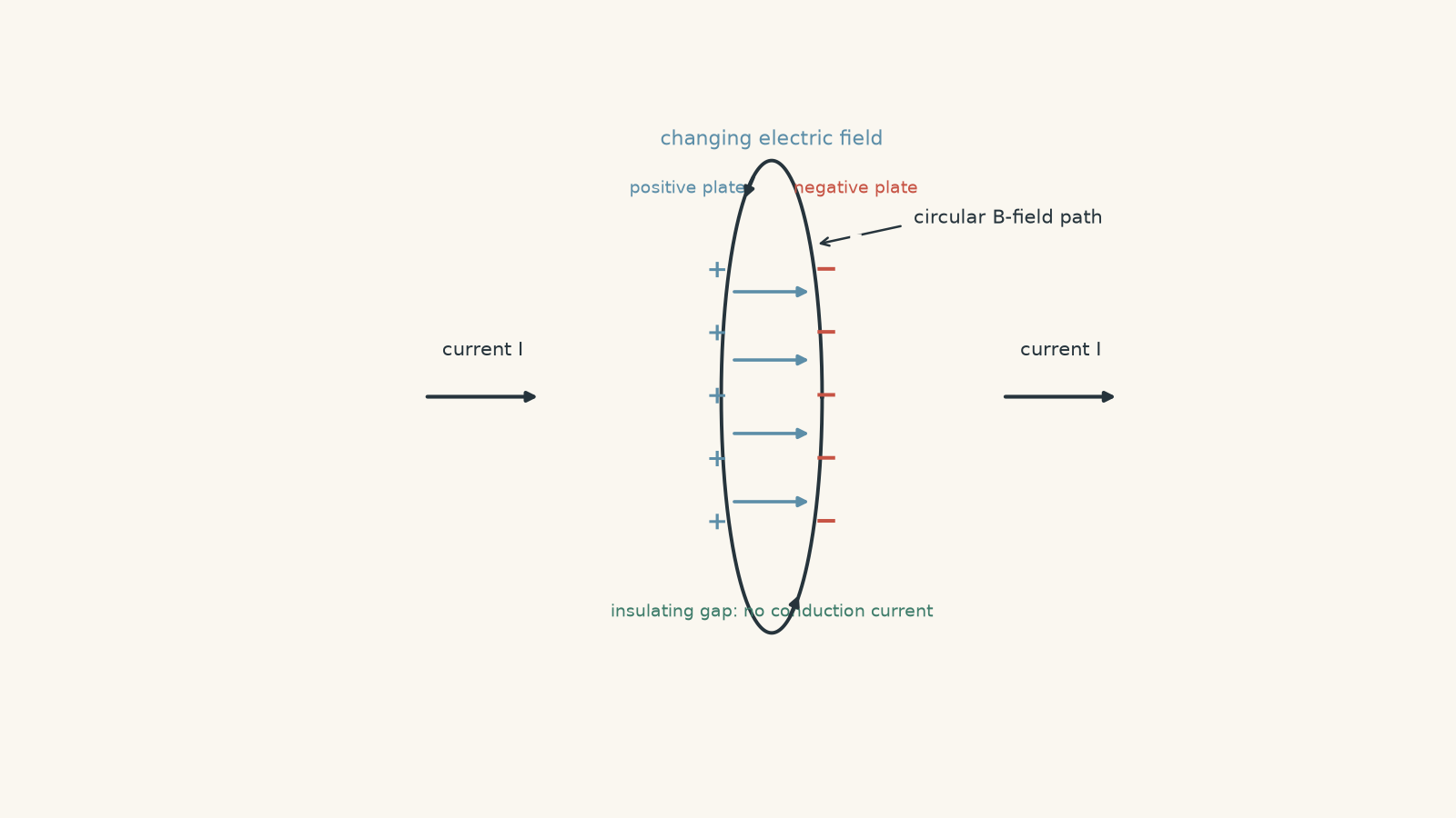
Now imagine a circular loop around the wire just before the capacitor.
Ampère’s original rule connected current with the magnetic field circulating around it. For a long straight wire,
\[
B(2\pi r)=\mu_0 I
\]
where \(B\) is the magnetic field at distance \(r\), \(I\) is the current, and \(\mu_0\) is the permeability of free space.
Here comes the problem.
Imagine stretching an invisible soap film across that circular loop. If the film cuts through the wire, current \(I\) passes through it, so Ampère’s rule predicts a magnetic field.
Now stretch the same imaginary soap film so that it bulges between the capacitor plates without cutting the wire. No conduction current crosses this second surface.
Should the same loop suddenly have \(B=0\)?
It cannot. The magnetic field at a point cannot depend on which imaginary surface you choose to draw.
The soap film is only bookkeeping, of course. It is useful because it exposes the contradiction in the old rule.
Maxwell’s correction was to recognise that the increasing electric field between the capacitor plates must also contribute to the surrounding magnetic field.
He introduced what is now called the displacement current:
\[
I_d=\epsilon_0\frac{\Delta\Phi_E}{\Delta t}
\]
for an average rate of change, where \(I_d\) is the displacement current, \(\epsilon_0\) is the permittivity of free space, and \(\Phi_E\) is electric flux.
Despite the name, this is not ordinary charge flowing through the gap. No tiny electrons are secretly leaping across an ideal capacitor. The changing electric field plays the role required by the magnetic-field equation.
A compact modern form of the Ampère-Maxwell law is
\[
\oint \mathbf{B}\cdot d\mathbf{l}
=
\mu_0\left(
I_{\text{cond}}
+
\epsilon_0\frac{d\Phi_E}{dt}
\right)
\]
The left side measures the magnetic field around a closed path. \(I_{\text{cond}}\) is the ordinary conduction current crossing a chosen surface, while the second term accounts for changing electric flux.
For an ideal charging capacitor, the displacement-current contribution between the plates matches the conduction current in the wire. The contradiction disappears.
Maxwell had supplied the other half of the link:
changing electric flux \(\rightarrow\) magnetic field
04What “unification” actually means
It is tempting to hear “Maxwell unified electricity and magnetism” and conclude that an electric field can never exist without a magnetic field.
That is not correct.
A stationary charged object can have a static electric field without a magnetic field in its own rest frame. A static magnetic field does not need a changing electric field beside it.
Electric and magnetic fields are not a clingy couple that must attend every event together.
The unification is in the laws connecting their sources and their changes.
| Situation | What Maxwell’s theory says |
|---|---|
| Static electric charge | Can produce a static electric field |
| Steady current | Produces a magnetic field |
| Changing magnetic flux | Produces a circulating electric field |
| Changing electric flux | Contributes to a circulating magnetic field |
| Travelling electromagnetic wave | Changing electric and magnetic fields propagate together |
That final row is the big one.
05How linked fields can form a travelling wave
Move far away from charges and currents. Suppose a disturbance in an electric field reaches some region of empty space.
Maxwell’s equations say that changes in the electric field are linked to the magnetic field pattern. Changes in the magnetic field are linked back to the electric field pattern.
The result can be a travelling solution: an electromagnetic wave.
This does not mean that an electric field at one point magically creates a magnetic field at exactly the same point, which then creates the electric field again in a little causal loop. Maxwell’s equations connect how fields vary across both space and time.
The whole field pattern propagates.
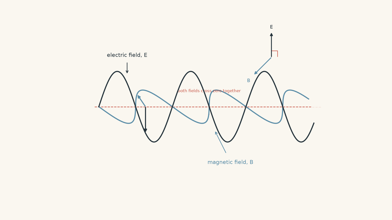
For an ideal plane electromagnetic wave in vacuum:
- the electric field \(\mathbf E\) is perpendicular to the magnetic field \(\mathbf B\)
- both fields are perpendicular to the direction of travel
- \(E\) and \(B\) oscillate in phase
- the wave travels at speed \(c\)
- the fields carry energy through space
For the field amplitudes,
\[
E_0=cB_0
\]
where \(E_0\) is the maximum electric field, \(B_0\) is the maximum magnetic field, and \(c\) is the speed of light.
Notice that \(E_0\) and \(B_0\) are not numerically equal. They have different units. The relationship involves \(c\).
Worked example: Maxwell predicts a wave speed
Using \(\mu_0=1.2566\times10^{-6}\ \mathrm{N\,A^{-2}}\) and \(\epsilon_0=8.854\times10^{-12}\) in SI units, calculate the speed Maxwell’s electromagnetic theory predicts for waves in vacuum.
Step 1
\[
c=\frac{1}{\sqrt{\mu_0\epsilon_0}}
\]
Here, \(\mu_0\) describes the magnetic properties appearing in the vacuum field equations, while \(\epsilon_0\) does the same for electric fields.
Step 2
\[
c=
\frac{1}
{\sqrt{
(1.2566\times10^{-6})
(8.854\times10^{-12})
}}
\]
Step 3
\[
c=
\frac{1}
{\sqrt{1.1126\times10^{-17}}}
=
\frac{1}{3.3356\times10^{-9}}
\]
Step 4
\[
c=2.998\times10^8\ \mathrm{m\,s^{-1}}
\]
This is the speed of light in vacuum.
That result is the heart of Maxwell’s argument. Constants that had appeared in apparently separate electrical and magnetic experiments produced the known speed of light.
Light was therefore not a completely different type of phenomenon. It could be understood as an electromagnetic wave.
06Why Maxwell’s speed prediction was such a powerful result
Suppose you were studying electricity and magnetism with no intention of explaining optics. You write down the laws of electric and magnetic fields and discover that they permit waves with speed
\[
\frac{1}{\sqrt{\mu_0\epsilon_0}}.
\]
You calculate the number.
It is the speed of light.
That is much stronger than simply noticing that electricity and light sometimes interact. The theory makes a quantitative prediction using electrical and magnetic constants, and that prediction lands on an independently measured property of light.
Maxwell’s theory therefore linked three subjects:
\[
\text{electricity}+\text{magnetism}+\text{light}
\rightarrow
\text{electromagnetism}.
\]
It also implied that visible light need not be the only possible electromagnetic wave. Other frequencies should be possible too.
Radio waves, microwaves, infrared, visible light, ultraviolet, X-rays, and gamma rays are not fundamentally different kinds of wave. They occupy different frequency and wavelength ranges of the electromagnetic spectrum.
07How an antenna actually produces the disturbance
A steady current can produce a steady magnetic field. That alone is not an electromagnetic wave travelling away through space.
To radiate strongly, charges must accelerate.
In a transmitting antenna, charges are driven backwards and forwards. As the charge distribution changes, the electric field around the antenna changes. The changing current also changes the magnetic field.
Those changing field patterns propagate outwards.
If the charges oscillate at frequency \(f\), the emitted electromagnetic wave has that same frequency. In vacuum,
\[
c=f\lambda
\]
where \(c\) is the wave speed in \(\mathrm{m\,s^{-1}}\), \(f\) is frequency in hertz (Hz), and \(\lambda\) is wavelength in metres (m).
Near a real antenna, the fields can be considerably more complicated than the neat textbook wave picture. Far enough from the source, the travelling-wave model becomes much more useful.
Worked example: A radio wave’s linked fields
A transmitter produces an electromagnetic wave of frequency \(100\ \mathrm{MHz}\) in vacuum. Its maximum electric field is \(120\ \mathrm{N\,C^{-1}}\). At one instant, the wave travels east while the electric field points north.
Calculate the wavelength and maximum magnetic field. State the direction of the magnetic field at that instant.
Step 1
\[
100\ \mathrm{MHz}
=
100\times10^6\ \mathrm{Hz}
=
1.00\times10^8\ \mathrm{Hz}
\]
Step 2
\[
\lambda=\frac{c}{f}
=
\frac{3.00\times10^8}
{1.00\times10^8}
=
3.00\ \mathrm{m}
\]
So successive identical points in the wave are \(3.00\ \mathrm{m}\) apart.
Step 3
\[
E_0=cB_0
\]
Therefore,
\[
B_0=\frac{E_0}{c}
=
\frac{120}
{3.00\times10^8}
=
4.00\times10^{-7}\ \mathrm{T}
\]
Step 4
For an electromagnetic wave, the direction of propagation is given by the direction of \(\mathbf E\times\mathbf B\).
The electric field points north and the wave travels east, so the magnetic field must point vertically upwards.
Half a cycle later, both fields reverse: \(E\) points south and \(B\) points down. Their cross-product still points east.
That is an important detail. The fields reverse together, so the wave does not reverse direction every half-cycle.
08The most tempting wrong picture: a quarter-cycle delay
A student often reasons like this:
“A changing electric field creates a magnetic field. So the magnetic field should be largest when the electric field is changing fastest. Therefore \(E\) and \(B\) should be \(90^\circ\) out of phase.”
It sounds sensible because it treats the relationship as though
\[
B\propto\frac{dE}{dt}.
\]
But Maxwell’s equations do not say that.
They connect the spatial variation of one field to the time variation of the other. A travelling wave depends on both.
For a sinusoidal plane wave moving in the \(+x\) direction, an acceptable form is
\[
E_y=E_0\cos(kx-\omega t)
\]
and
\[
B_z=B_0\cos(kx-\omega t),
\]
where \(k\) describes how rapidly phase changes with position and \(\omega\) describes how rapidly phase changes with time.
The cosine factors are identical. The two fields are in phase.
At a particular location, when \(E\) reaches a maximum, its instantaneous rate of change is zero. That does not mean the magnetic field must disappear. It means the student has confused a field’s value with one derivative appearing in a field equation.
A travelling wave is a pattern spread through space, not two local numbers taking turns creating each other.
09Another misconception: the fields generate free energy
If each changing field helps sustain the other, it can sound as though the wave produces its own energy forever.
It does not.
The energy comes from the source that accelerated the charges in the first place. A transmitting antenna draws electrical energy from its power supply and transfers some of that energy into the electromagnetic field.
Once launched, the wave transports that energy.
For a spherical wave spreading away from a source, its energy is distributed over a growing area, so the field amplitudes generally fall with distance. Maxwell’s coupling laws describe how the fields propagate; they are not an energy-creation machine.
Physics remains disappointingly resistant to free electricity.
10The idea to keep
You do not need to reduce Maxwell’s unification to “electricity makes magnetism”.
A better chain is:
\[
\text{charges and currents produce fields}
\]
\[
\text{changing magnetic fields are linked to electric fields}
\]
\[
\text{changing electric fields are linked to magnetic fields}
\]
\[
\text{the coupled field equations allow waves}
\]
\[
\text{their predicted speed is }c
\]
\[
\therefore\text{ light is an electromagnetic wave.}
\]
That is the useful mental model.
11Questions and solutions
Question 1
A positively charged conducting sphere is held stationary in a laboratory.
A student says, “Maxwell unified electricity and magnetism, so the sphere must produce both an electric field and a magnetic field.”
Is the student’s conclusion correct? Explain what Maxwell’s unification actually requires.
Solution 1
No. The stationary charged sphere can produce a static electric field without producing a magnetic field in its rest frame.
The sphere has charge, so it creates an electric field around itself. Because the charge distribution is stationary, there is no ordinary current associated with that sphere and no requirement for a magnetic field to accompany its static electric field.
The tempting mistake is to interpret “unified” as “always present together”.
Maxwell’s unification is more precise. Electric and magnetic fields obey one connected set of laws. In particular, changing magnetic fields are linked with electric fields, and changing electric flux contributes to magnetic fields.
An electromagnetic wave is one important situation in which changing electric and magnetic fields travel together. A static charged sphere is not an electromagnetic wave.
Question 2
An ideal parallel-plate capacitor has plate area
\[
A=2.0\times10^{-2}\ \mathrm{m^2}.
\]
While it is charging, the electric field between its plates increases uniformly at
\[
\frac{\Delta E}{\Delta t}
=
1.5\times10^{12}\ \mathrm{V\,m^{-1}\,s^{-1}}.
\]
Use
\[
\epsilon_0=8.85\times10^{-12}
\]
in SI units.
Assume the field between the plates is uniform and negligible outside them.
Calculate the displacement current using
\[
I_d=\epsilon_0 A\frac{\Delta E}{\Delta t}.
\]
Hence state the conduction current in the wire. Explain why this does not mean charge is conducting through the insulating gap.
Solution 2
The displacement current is \(0.266\ \mathrm{A}\), so the ideal conduction current in the connecting wire is also \(0.266\ \mathrm{A}\); this does not require charges to cross the capacitor gap.
The electric flux through one plate is \(\Phi_E=EA\) because the field is uniform and perpendicular to the plate.
Therefore,
\[
I_d
=
\epsilon_0 A\frac{\Delta E}{\Delta t}.
\]
Substituting,
\[
\begin{aligned}
I_d
&=
(8.85\times10^{-12})
(2.0\times10^{-2})
(1.5\times10^{12})\\
&=0.2655\ \mathrm{A}\\
&\approx0.266\ \mathrm{A}.
\end{aligned}
\]
For an ideal charging capacitor,
\[
I_{\text{wire}}=I_d,
\]
so
\[
I_{\text{wire}}\approx0.266\ \mathrm{A}.
\]
The tempting interpretation is that “displacement current” must mean charge crosses the gap at \(0.266\ \mathrm{C\,s^{-1}}\).
It does not. Ordinary conduction current reaches the plates and changes the charge stored on them. That changing charge changes the electric field between the plates.
Maxwell’s displacement-current term accounts for that changing electric flux in the magnetic-field law. It gives the same magnetic-field prediction whether an imaginary surface cuts the conducting wire or passes through the capacitor gap.
That consistency is the entire point of the correction.
Question 3
A transmitter produces a continuous electromagnetic wave of frequency \(120\ \mathrm{MHz}\) in vacuum.
Two detectors, A and B, lie on the same line away from the transmitter. B is \(15.0\ \mathrm{m}\) farther from the transmitter than A.
The sinusoidal signals recorded at A and B happen to be in phase.
A student argues that this proves both detectors respond to the transmitter simultaneously.
Calculate:
- the wavelength of the radiation
- the number of wavelengths separating A and B
- the extra travel time for a sudden modulation pulse to reach B after A
Then explain why the student’s interpretation is wrong.
Solution 3
The wavelength is \(2.50\ \mathrm{m}\), the detectors are separated by exactly six wavelengths, and a new modulation reaches B \(50.0\ \mathrm{ns}\) after it reaches A. Their signals can therefore be in phase without the electromagnetic influence travelling instantaneously.
First convert the frequency:
\[
f=120\ \mathrm{MHz}
=
1.20\times10^8\ \mathrm{Hz}.
\]
Using
\[
c=f\lambda,
\]
we get
\[
\lambda
=
\frac{c}{f}
=
\frac{3.00\times10^8}
{1.20\times10^8}
=
2.50\ \mathrm{m}.
\]
The separation in wavelengths is
\[
\frac{15.0}{2.50}=6.00.
\]
So detector B is exactly six wavelengths farther along the propagation direction.
A shift of one whole wavelength corresponds to a phase shift of \(360^\circ\). Six wavelengths correspond to
\[
6(360^\circ)=2160^\circ,
\]
which is equivalent to a net phase difference of \(0^\circ\).
That explains why the continuous sinusoidal signals can look in phase.
Now calculate the propagation delay:
\[
\Delta t
=
\frac{\Delta x}{c}
=
\frac{15.0}
{3.00\times10^8}
=
5.00\times10^{-8}\ \mathrm{s}.
\]
Therefore,
\[
\Delta t=50.0\ \mathrm{ns}.
\]
The tempting route is to use “same phase” as evidence for “same time”.
Phase does not tell you how many whole cycles separate two points. B can be six complete wavelengths behind A and still have exactly the same instantaneous field direction.
A sudden change in the transmitted signal exposes the propagation time: the change reaches A first and B \(50.0\ \mathrm{ns}\) later.
Maxwell’s fields propagate at finite speed.
Question 4
An ideal plane electromagnetic wave travels in the \(+x\) direction through vacuum. At a particular instant and location,
- the electric field points in the \(+y\) direction
- \(E=240\ \mathrm{N\,C^{-1}}\)
- a proton is moving in the \(+x\) direction at \(0.75c\)
Use \(q_p=1.60\times10^{-19}\ \mathrm{C}\) and \(E=cB\).
Determine:
- the magnitude and direction of the magnetic field
- the electric force on the proton
- the magnetic force on the proton
- the net electromagnetic force at that instant
Then determine the net force if the same proton were instead moving at \(0.75c\) in the \(-x\) direction.
Finally, a student claims that a co-propagating proton could make the electric and magnetic forces cancel completely by travelling fast enough. Evaluate that claim.
Solution 4
For the proton moving with the wave at \(0.75c\), the magnetic force opposes the electric force and the net force is \(9.6\times10^{-18}\ \mathrm{N}\) in the \(+y\) direction. For motion against the wave, the two forces add. Complete cancellation for a co-propagating proton would require \(v=c\), which a proton cannot reach.
First find the magnetic field.
For a plane electromagnetic wave,
\[
E=cB,
\]
so
\[
B=\frac{E}{c}.
\]
Substituting,
\[
B
=
\frac{240}
{3.00\times10^8}
=
8.00\times10^{-7}\ \mathrm{T}.
\]
The wave travels in \(+x\), while \(\mathbf E\) points in \(+y\). The magnetic field must point in \(+z\), because
\[
\mathbf E\times\mathbf B
\]
must point in the direction of propagation.
The electric force is
\[
F_E=qE.
\]
Therefore,
\[
F_E
=
(1.60\times10^{-19})(240)
=
3.84\times10^{-17}\ \mathrm{N}.
\]
Because the proton is positive, this force points in \(+y\).
For the proton travelling in \(+x\),
\[
F_B=qvB
\]
because the velocity is perpendicular to the magnetic field.
Using \(v=0.75c\),
\[
\begin{aligned}
F_B
&=
q(0.75c)\left(\frac{E}{c}\right)\\
&=0.75qE\\
&=0.75(3.84\times10^{-17})\\
&=2.88\times10^{-17}\ \mathrm{N}.
\end{aligned}
\]
The magnetic-force direction comes from \(\mathbf v\times\mathbf B\).
Here,
\[
(+x)\times(+z)=-y,
\]
so the magnetic force points in \(-y\).
The forces therefore oppose:
\[
F_{\text{net}}
=
F_E-F_B.
\]
Thus,
\[
\begin{aligned}
F_{\text{net}}
&=
3.84\times10^{-17}
–
2.88\times10^{-17}\\
&=
9.6\times10^{-18}\ \mathrm{N}.
\end{aligned}
\]
The net force points in \(+y\).
Now reverse the proton’s velocity.
For motion in \(-x\),
\[
(-x)\times(+z)=+y.
\]
The magnetic force now points in the same direction as the electric force.
Its magnitude is still \(2.88\times10^{-17}\ \mathrm{N}\), so
\[
\begin{aligned}
F_{\text{net}}
&=
3.84\times10^{-17}
+
2.88\times10^{-17}\\
&=
6.72\times10^{-17}\ \mathrm{N}
\end{aligned}
\]
in \(+y\).
The student’s final idea has an interesting piece of correct algebra inside it.
For a proton travelling with the wave,
\[
F_{\text{net}}=qE-qvB.
\]
Since \(B=E/c\),
\[
F_{\text{net}}
=
qE\left(1-\frac{v}{c}\right).
\]
The forces would cancel if
\[
1-\frac{v}{c}=0,
\]
so
\[
v=c.
\]
But a proton has non-zero rest mass and cannot be accelerated to the speed of light.
The deeper trap is assuming that because the electric and magnetic fields belong to the same electromagnetic wave, their forces on a moving charge must point together. Magnetic force depends on the charge’s velocity as well as the field. Changing the particle’s direction can change the magnetic-force direction even though the wave itself is unchanged.
Question 5
Two students are trying to sketch an ideal sinusoidal electromagnetic wave travelling through vacuum in the \(+x\) direction.
Both use
\[
E_y=E_0\cos(kx-\omega t).
\]
Student A argues:
“Magnetic field is produced by a changing electric field. Therefore \(B\) should be greatest when \(E\) changes fastest.”
A therefore proposes
\[
B_z=B_0\sin(kx-\omega t),
\]
putting the two fields a quarter-cycle out of phase.
Student B proposes
\[
B_z=B_0\cos(kx-\omega t),
\]
so the fields are in phase.
Determine which student has the correct travelling-wave model.
Then resolve this apparent contradiction: at a position and instant where \(E\) is maximum, its instantaneous rate of change with time is zero. If the magnetic field supposedly depends on the changing electric field, why can \(B\) also be maximum there rather than zero?
Finally, does your conclusion mean that every possible electric and magnetic field configuration must always have \(E\) and \(B\) in phase?
Solution 5
Student B has the correct model for an ideal plane electromagnetic wave travelling through vacuum: the electric and magnetic fields are in phase. The apparent contradiction disappears because Maxwell’s equations do not state that the magnetic-field magnitude is proportional to the local time derivative of the electric-field magnitude. They connect changes across both space and time. The in-phase result also does not apply to every possible electromagnetic field configuration.
For the travelling wave,
\[
E_y=E_0\cos(kx-\omega t)
\]
and
\[
B_z=B_0\cos(kx-\omega t),
\]
with
\[
E_0=cB_0.
\]
Both fields therefore reach positive maxima together, pass through zero together, reach negative maxima together, and reverse together.
Student A’s argument is tempting because the phrase “a changing electric field produces a magnetic field” sounds like the simple relationship
\[
B\propto\frac{\partial E}{\partial t}.
\]
If that were Maxwell’s rule, Student A’s quarter-cycle shift would make sense.
But that is not the rule.
Maxwell’s equations connect the time variation of one field to how the other field varies from place to place. In a travelling wave, the spatial and temporal structures are linked through the travelling phase
\[
kx-\omega t.
\]
You cannot correctly analyse the wave by watching the time dependence at one isolated point and ignoring the neighbouring field pattern.
Now consider an electric-field maximum.
For a cosine wave, the instantaneous time derivative is zero at a maximum. That is ordinary sinusoidal behaviour: anything oscillating smoothly has zero instantaneous slope as it turns around at a peak.
The magnetic field can simultaneously be at its own maximum because Maxwell’s equations never required
\[
B=0
\]
whenever
\[
\frac{\partial E}{\partial t}=0.
\]
The field values and the rates at which those values change are different quantities.
A useful comparison is an object thrown vertically upwards. At its highest point, its instantaneous velocity is zero. That does not mean gravity has vanished or the entire motion has stopped permanently. The zero is describing one instantaneous rate, not the complete physical state.
The analogy breaks if taken too far because an electromagnetic wave is a field distributed through space, not a projectile. Its real lesson is simply that “zero rate of change right now” does not mean “nothing exists” or “nothing can happen next”.
Finally, \(E\) and \(B\) being in phase is a property of the ideal travelling plane wave considered here. It is not a rule that every electric and magnetic field everywhere must share the same phase. Static fields, fields close to complicated sources, and standing-wave arrangements need not behave like a single travelling plane wave.
That distinction is the conceptual payoff of Maxwell’s unification. The theory does not give you a slogan saying electricity and magnetism always copy one another. It gives you precise relationships between fields across space and time.
Once those relationships predict a universal electromagnetic wave speed \(c\), the next question becomes unavoidable: what happens to that speed when the observer moves? Following that question leads directly from Maxwell’s electromagnetism into special relativity.