
Maxwell’s Prediction of Electromagnetic Waves: HSC Physics
Learn how Maxwell showed that changing electric and magnetic fields can form a self-propagating electromagnetic wave. Includes worked examples, misconceptions, and challenging HSC-style questions.
A radio transmitter can send energy across kilometres of empty space. There is no wire between the transmitter and your radio, and there does not need to be air in between. So what is actually travelling?
Before Maxwell, electricity and magnetism could look like two related but separate topics. Charges produce electric fields. Currents produce magnetic fields. Faraday had also shown that a changing magnetic field can produce an electric effect.
Now make a prediction. If a changing magnetic field can create an electric field, could a changing electric field create a magnetic field in return?
Maxwell realised that it had to. Once that missing piece was added, the equations allowed something remarkable: a disturbance in the electric and magnetic fields could propagate through empty space as a wave.
That wave is electromagnetic radiation. Light is one example.
01The problem Maxwell had to solve
Start with two established ideas.
A stationary charge produces an electric field. A steady current produces a magnetic field.
Faraday’s experiments added something less obvious: when magnetic flux changes, an electric field appears. This is the physics behind electromagnetic induction.
You can review how Maxwell brought these ideas together in Maxwell’s unification of electricity and magnetism.
But there was an asymmetry.
A changing magnetic field could produce an electric field, yet the equations describing magnetism originally treated electric current as the only source of a circulating magnetic field.
Maxwell suspected that this was incomplete.
02A capacitor exposes the problem
Imagine a capacitor being charged by a battery.
Current flows through the wires towards one capacitor plate. Electrons accumulate on one plate and leave the other.
But no charge crosses the insulating gap between the plates.
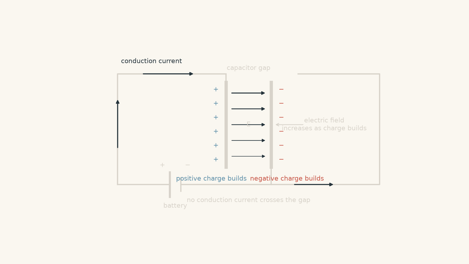
Now imagine drawing a loop around the wire and asking what produces the magnetic field around that loop.
If you stretch an imaginary surface across the loop so that it cuts through the wire, current passes through the surface.
No problem.
But you could instead stretch the same surface out between the capacitor plates. No conduction current passes through that surface.
The magnetic field cannot depend on which imaginary surface you happen to choose. Maxwell therefore needed something in the capacitor gap that played the magnetic role of a current.
There was: the electric field between the plates was changing.
Maxwell added a term associated with changing electric flux. It is commonly called the displacement current term.
The important HSC idea is simpler than the name makes it sound:
A changing electric field produces a magnetic field.
This completes the symmetry we need for electromagnetic waves.
03How can fields form a travelling wave?
Picture a transmitter antenna in which charges are accelerating back and forth.
The motion creates a changing electric field around the antenna.
That changing electric field is associated with a changing magnetic field.
The magnetic field also changes, so Faraday’s law tells us that a circulating electric field is produced.
The disturbance does not stay beside the antenna. Maxwell’s equations permit the coupled electric and magnetic fields to propagate outwards.
A useful first picture is a stadium wave. One person moves, then nearby people respond, then people farther along respond. The pattern travels even though the individual people do not travel around the stadium.
For an electromagnetic wave, it is the electromagnetic disturbance that moves through space.
The analogy has an important limit. People in a stadium respond because they see their neighbours. Electric and magnetic fields are not little objects watching one another. The exact description is given by Maxwell’s equations: spatial and temporal changes in the fields are coupled in a way that permits a propagating wave.
04The two key pieces
For an electromagnetic wave travelling through empty space:
- A changing magnetic field is associated with a circulating electric field.
- A changing electric field is associated with a circulating magnetic field.
The first comes from Faraday’s law. The second comes from Maxwell’s correction to Ampère’s law.
This is often summarised by saying that changing electric and magnetic fields “sustain each other”.
That phrase is useful, but it needs care. It does not mean that an electric field disappears, waits, and then manufactures a magnetic field, which later manufactures a new electric field.
Both fields are parts of one electromagnetic system. Maxwell’s equations describe how their values vary together through space and time.
05What does the wave look like?
Suppose an electromagnetic wave travels in the \(x\)-direction.
Its electric field might oscillate in the \(y\)-direction, while its magnetic field oscillates in the \(z\)-direction.
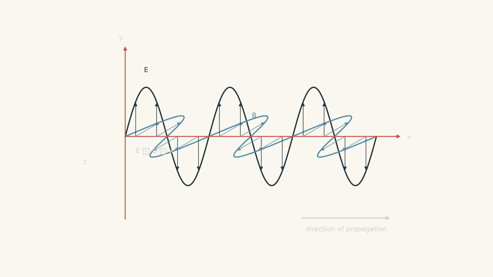
The three directions are perpendicular:
- the electric field \(\vec E\),
- the magnetic field \(\vec B\), and
- the direction in which the wave travels.
So electromagnetic waves are transverse waves.
For a plane electromagnetic wave in vacuum, the direction of propagation is given by the direction of
\[
\vec E \times \vec B
\]
where \(\vec E\) is the electric field and \(\vec B\) is the magnetic field.
You do not need to imagine the fields physically waving like ropes. The arrows representing field strength and direction vary from place to place and from moment to moment.
06Maxwell’s astonishing prediction
Once Maxwell included the changing-electric-field term, his equations predicted that electromagnetic disturbances should travel with speed
\[
v=\frac{1}{\sqrt{\mu_0\varepsilon_0}}
\]
where:
- \(v\) is the predicted wave speed in metres per second,
- \(\mu_0\) is the permeability of free space, and
- \(\varepsilon_0\) is the permittivity of free space.
Using
\[
\mu_0 = 4\pi\times10^{-7}\ \text{T m A}^{-1}
\]
and approximately
\[
\varepsilon_0 = 8.85\times10^{-12}\ \text{F m}^{-1},
\]
the predicted speed is about
\[
3.00\times10^8\ \text{m s}^{-1}.
\]
That was already known to be approximately the speed of light.
The conclusion was enormous: light could be an electromagnetic wave.
Radio waves, microwaves, infrared, visible light, ultraviolet, X-rays, and gamma rays are now all understood as electromagnetic radiation. They differ in frequency and wavelength, not in the basic mechanism of propagation through vacuum.
Worked example: Calculate Maxwell’s predicted wave speed
Use \(\mu_0=4\pi\times10^{-7}\ \text{T m A}^{-1}\) and \(\varepsilon_0=8.85\times10^{-12}\ \text{F m}^{-1}\) to calculate the speed predicted for an electromagnetic wave in vacuum.
Step 1
\[
v=\frac{1}{\sqrt{\mu_0\varepsilon_0}}
\]
Step 2
\[
v=
\frac{1}{
\sqrt{
(4\pi\times10^{-7})
(8.85\times10^{-12})
}
}
\]
The product is approximately
\[
(4\pi\times10^{-7})(8.85\times10^{-12})
\approx1.11\times10^{-17}.
\]
So
\[
v\approx
\frac{1}{\sqrt{1.11\times10^{-17}}}
\approx3.00\times10^8\ \text{m s}^{-1}.
\]
Step 3
The predicted speed is
\[
v\approx3.00\times10^8\ \text{m s}^{-1},
\]
which matches the speed of light in vacuum.
Maxwell therefore had a strong theoretical reason to identify light as an electromagnetic wave.
07The fields are linked in size as well as direction
For an electromagnetic wave in vacuum, the magnitudes of the electric and magnetic fields satisfy
\[
E=cB,
\]
or equivalently,
\[
\frac{E}{B}=c,
\]
where:
- \(E\) is the electric field magnitude in \(\text{V m}^{-1}\),
- \(B\) is the magnetic field magnitude in tesla,
- \(c\) is the speed of light in vacuum, approximately \(3.00\times10^8\ \text{m s}^{-1}\).
This tells you something important.
The electric and magnetic parts are not independent waves that happen to travel beside each other. Their magnitudes are linked.
Worked example: Find the magnetic field in a radio wave
At one instant, the electric field in a radio wave in vacuum has magnitude \(24.0\ \text{V m}^{-1}\). Calculate the magnetic field magnitude at the same point and instant.
Step 1
\[
E=cB
\]
Rearrange for \(B\):
\[
B=\frac{E}{c}.
\]
Step 2
\[
B=
\frac{24.0\ \text{V m}^{-1}}
{3.00\times10^8\ \text{m s}^{-1}}
=8.00\times10^{-8}\ \text{T}.
\]
Step 3
The magnetic field magnitude is
\[
B=8.00\times10^{-8}\ \text{T}.
\]
That looks tiny compared with the electric-field number, but comparing the numerical sizes directly is misleading because \(E\) and \(B\) have different units.
08Why accelerating charges matter
A common shortcut is to say, “moving charges produce electromagnetic waves”.
That is too broad.
A charge moving at constant velocity has electric and magnetic fields, but steady uniform motion by itself is not the same as continuously radiating an electromagnetic wave.
Radiation is associated with accelerating charges.
In a transmitting antenna, charges oscillate back and forth. Their velocity is constantly changing, so they are accelerating.
That produces a time-varying electromagnetic disturbance that can propagate away from the source.
This is why an alternating current can be used in a radio transmitter. The oscillating charges generate electromagnetic radiation at the driving frequency.
09Why the wave does not need a medium
Mechanical waves involve matter.
A sound wave is a disturbance in the positions and pressures of particles in a material. Remove the material, and there are no particles to carry the sound.
It would therefore have been natural to predict that light also needed some invisible material to vibrate.
Maxwell’s equations suggested otherwise.
The quantities changing in an electromagnetic wave are the electric and magnetic fields themselves. The wave can therefore propagate through vacuum.
That does not mean there is “nothing happening” in empty space. The electromagnetic field has measurable properties and carries energy and momentum.
10The most tempting misconception
A common diagram shows a sinusoidal electric field and a sinusoidal magnetic field crossing at right angles. It is easy to look at that diagram and imagine this sequence:
electric field peaks → magnetic field starts growing → magnetic field peaks → electric field starts growing again.
That is not what a plane electromagnetic wave does.
At a particular location in an ideal sinusoidal electromagnetic wave, \(E\) and \(B\) reach zero together and reach their maximum magnitudes together. They are in phase.
So how can changing fields be involved if both fields are maximum at the same time?
Because Maxwell’s equations involve changes across both time and space.
At a field maximum, the instantaneous time rate of change at that exact point can be zero, while the spatial structure of the travelling wave still satisfies the coupled field equations.
The phrase “one changing field creates the other” is therefore a useful introduction, not a frame-by-frame mechanical story.
11Frequency, wavelength, and speed
Once electromagnetic radiation is recognised as a wave, the familiar wave relationship applies:
\[
v=f\lambda,
\]
where:
- \(v\) is wave speed in \(\text{m s}^{-1}\),
- \(f\) is frequency in hertz,
- \(\lambda\) is wavelength in metres.
In vacuum,
\[
c=f\lambda.
\]
The speed is fixed at \(c\), so increasing the frequency decreases the wavelength.
Worked example: Connect an antenna frequency to wavelength
A transmitter produces electromagnetic radiation with frequency \(100\ \text{MHz}\). Calculate its wavelength in vacuum.
Step 1
Since \(1\ \text{MHz}=10^6\ \text{Hz}\),
\[
f=100\times10^6\ \text{Hz}
=1.00\times10^8\ \text{Hz}.
\]
Step 2
\[
c=f\lambda.
\]
Rearrange:
\[
\lambda=\frac{c}{f}.
\]
Step 3
\[
\lambda=
\frac{3.00\times10^8\ \text{m s}^{-1}}
{1.00\times10^8\ \text{s}^{-1}}
=3.00\ \text{m}.
\]
The wavelength is therefore
\[
\lambda=3.00\ \text{m}.
\]
A \(100\ \text{MHz}\) signal has a wavelength of about three metres in vacuum.
12What Maxwell actually predicted
It helps to separate three claims.
| Claim | Status |
|---|---|
| Changing magnetic fields are associated with electric fields | Established through electromagnetic induction |
| Changing electric fields are associated with magnetic fields | Maxwell’s crucial addition to the existing theory |
| The coupled equations permit waves travelling at \(1/\sqrt{\mu_0\varepsilon_0}\) | Mathematical consequence of Maxwell’s theory |
The predicted speed agreed with the measured speed of light.
Later experiments, particularly Hertz’s production and detection of radio waves, provided direct experimental evidence for electromagnetic waves beyond visible light.
Maxwell’s achievement was therefore not simply noticing that light was fast. His equations linked electricity, magnetism, and optics within one theory and predicted electromagnetic waves as a consequence.
13Questions and solutions
Question 1
An electromagnetic wave travels through vacuum. Its electric field has a maximum magnitude of \(150\ \text{V m}^{-1}\).
Calculate the maximum magnetic field magnitude.
Solution 1
The maximum magnetic field is \(5.00\times10^{-7}\ \text{T}\).
For an electromagnetic wave in vacuum,
\[
E=cB.
\]
Rearranging,
\[
B=\frac{E}{c}.
\]
Substitute \(E=150\ \text{V m}^{-1}\) and \(c=3.00\times10^8\ \text{m s}^{-1}\):
\[
B=
\frac{150}
{3.00\times10^8}
=5.00\times10^{-7}\ \text{T}.
\]
So
\[
B=5.00\times10^{-7}\ \text{T}.
\]
The tempting mistake is to treat \(E\) and \(B\) as unrelated amplitudes. In a plane electromagnetic wave in vacuum, their magnitudes are constrained by \(E/B=c\).
Question 2
A student says:
“An electromagnetic wave must eventually die in vacuum because the electric field uses some of its energy creating the magnetic field, then the magnetic field uses more energy recreating the electric field.”
Explain why this model is incorrect. Your answer should refer to both Maxwell’s equations and energy conservation.
Solution 2
The model is incorrect because the electric and magnetic fields are coupled components of one propagating electromagnetic field, not two systems repeatedly spending energy to recreate each other.
Maxwell’s equations relate spatial and temporal variations of \(\vec E\) and \(\vec B\). In vacuum, these coupled equations admit travelling-wave solutions.
The phrase “a changing electric field creates a magnetic field, which creates an electric field” is useful for building intuition, but it becomes misleading if interpreted as a repeated energy-payment process.
An ideal electromagnetic wave travelling through vacuum does not lose energy merely because its electric and magnetic fields vary. Energy is transported by the electromagnetic field.
If the wave interacts with matter, energy can be absorbed, scattered, or otherwise transferred. But vacuum propagation itself does not require the wave to continuously sacrifice energy to keep existing.
The tempting route is to imagine two fields taking turns like two people lending the same twenty-dollar note back and forth while somehow paying a fee each time. Maxwell’s equations do not describe that process. They describe one coupled field configuration moving through space.
Question 3
A plane electromagnetic wave travels east. At one instant and position, its electric field points vertically upwards.
Determine the direction of its magnetic field. Explain how you know.
Solution 3
The magnetic field must point horizontally towards either north or south depending on the coordinate convention, with the correct choice being the direction that makes \(\vec E\times\vec B\) point east.
Take east as \(+x\), north as \(+y\), and up as \(+z\).
The electric field points up, so
\[
\vec E\parallel +z.
\]
We require
\[
\vec E\times\vec B\parallel +x.
\]
Using the right-hand rule,
\[
\hat z\times(-\hat y)=\hat x.
\]
Therefore the magnetic field points south.
So the three directions are mutually perpendicular:
- \(\vec E\): up,
- \(\vec B\): south,
- propagation: east.
The tempting mistake is to say only that the magnetic field must be perpendicular to the electric field. That is necessary but not sufficient. Both north and south are perpendicular to up. The propagation direction selects the correct one through \(\vec E\times\vec B\).
Question 4
Two transmitters are proposed.
Transmitter A contains charges oscillating sinusoidally back and forth.
Transmitter B somehow sends a group of charges through a long straight section of apparatus at constant velocity, with the number of charges passing each point per second remaining constant.
A student argues that both must radiate continuously because both involve moving charges and therefore both produce magnetic fields.
Assess this argument. Explain what is fundamentally different between the electromagnetic fields of the two systems.
Solution 4
Only Transmitter A necessarily has the time-varying source behaviour required for continuous electromagnetic radiation; the student’s argument confuses the existence of a magnetic field with the production of a propagating electromagnetic wave.
In Transmitter A, the charges oscillate. Their velocities continually change, which means they accelerate.
The resulting charge and current distribution varies with time. The electromagnetic field around the source therefore changes, and part of that changing field can propagate away as electromagnetic radiation.
Transmitter B is different. In the idealised steady situation described, the current at each point is constant with time. The system can have a magnetic field because moving charge constitutes current, but a steady magnetic field is not itself an outgoing electromagnetic wave.
The crucial distinction is therefore not
\[
\text{charge moving} \quad \text{versus} \quad \text{charge stationary}.
\]
It is whether the source produces the changing electromagnetic configuration associated with radiation.
There is one subtlety. Individual charges entering, leaving, or being redirected by a real apparatus must accelerate somewhere, and those regions may radiate. But the question specifies the long straight section with constant velocity and constant current. That steady section is not continuously radiating merely because a magnetic field exists around it.
The tempting route is:
\[
\text{moving charge}\rightarrow\text{magnetic field}\rightarrow\text{electromagnetic wave}.
\]
The missing constraint is that a static or steady field is not the same thing as a propagating disturbance. Electromagnetic radiation is associated with time-varying source behaviour, particularly accelerating charges.
Question 5
Consider an ideal plane electromagnetic wave travelling through vacuum in the \(+x\)-direction. At position \(x=0\), the electric field is described by
\[
E_y=E_0\cos(\omega t).
\]
A student looks at the instant \(t=0\) and argues:
“The electric field is at its maximum, so \(dE/dt=0\). Therefore the electric field is not changing. Maxwell says a changing electric field produces a magnetic field, so the magnetic field must be zero at this instant.”
Yet for a plane electromagnetic wave, the magnetic field is actually at its maximum magnitude at the same place and time.
Resolve the apparent contradiction without dismissing either statement. Explain why considering only \(dE/dt\) at one point gives an incomplete picture of Maxwell’s theory.
Solution 5
There is no contradiction: the magnetic field can be maximum when the electric field is maximum because Maxwell’s equations connect changes in both time and space, not simply the value of \(dE/dt\) at one isolated point.
For a travelling plane wave, the electric field has a form such as
\[
E_y(x,t)=E_0\cos(kx-\omega t),
\]
where:
- \(E_0\) is the maximum electric field,
- \(k\) is the wave number,
- \(x\) is position,
- \(\omega\) is angular frequency,
- \(t\) is time.
The associated magnetic field is in phase with it:
\[
B_z(x,t)=B_0\cos(kx-\omega t).
\]
At \(x=0\) and \(t=0\),
\[
E_y=E_0
\]
and
\[
B_z=B_0.
\]
Both fields are therefore at their maximum values.
It is also true that the time derivative of \(E_y\) at that exact event is zero:
\[
\frac{\partial E_y}{\partial t}
=
\omega E_0\sin(kx-\omega t),
\]
so at \(x=0,\ t=0\),
\[
\frac{\partial E_y}{\partial t}=0.
\]
The student’s error is assuming that the magnetic field at a point is determined simply by the instantaneous time derivative of the electric field at exactly the same point.
Maxwell’s equations are spatial field equations. For example, they connect how fields curl through space with how other fields change in time. A travelling electromagnetic wave therefore has to be considered as a complete pattern across neighbouring positions, not as one isolated arrow observed at one instant.
At the crest, the field value is maximum and its instantaneous time rate of change at that point is zero. A fraction of a period later, the crest has moved. The entire spatial pattern satisfies Maxwell’s equations continuously.
This is the deeper correction to the simplified phrase “changing electric fields make magnetic fields”. That phrase points in the right direction, but the exact physics is a coupled relationship between the spatial and temporal variation of both fields.
Once that distinction is clear, Maxwell’s prediction becomes much more powerful. The theory does not merely explain why electric and magnetic effects are related. It predicts a travelling electromagnetic structure, fixes its speed in vacuum, links the sizes and directions of its fields, and provides the foundation for understanding how antennas generate radiation and how electromagnetic waves carry energy through space.