
Finding Stellar Temperature from Spectra: HSC Physics
Learn how spectrum shape, Wien’s law, and absorption-line strength can be used together to estimate stellar surface temperature.
Two stars can look almost equally bright through a telescope, yet one is blue-white and the other orange. Which one has the hotter surface?
Your first prediction is probably the blue-white star. That is usually right, but colour alone is a rough clue. A spectrum gives us much more: a smooth distribution of light across wavelength, with narrow absorption lines cut into it. The shape of that smooth background and the pattern of the lines both contain information about temperature, but they tell us in different ways.
The important HSC skill is knowing which clue means what.
01Start with the shape of the spectrum
Imagine plotting the intensity of a star’s light against wavelength. Instead of giving equal amounts of every wavelength, the star produces a broad hump.
The wavelength at the top of that hump is called the peak wavelength, \(\lambda_{\text{max}}\).
Now make a prediction. If a star becomes hotter, would you expect its peak to move towards longer, redder wavelengths, or shorter, bluer wavelengths?
It moves towards shorter wavelengths.
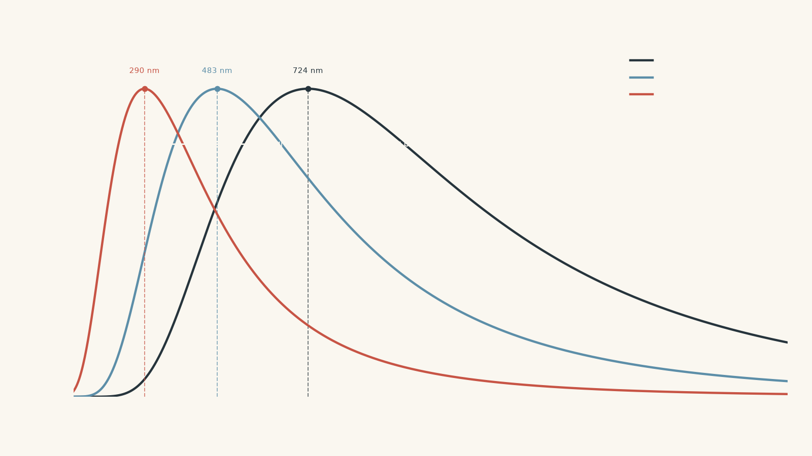
A useful first model is to treat a star as a hot object emitting thermal radiation. A cooler object produces proportionally more long-wavelength radiation. Raise its temperature, and the distribution shifts towards shorter wavelengths.
This is why very hot stars tend to look blue-white, while cooler stars tend to look orange or red.
But “blue means hot” is only the starting model. We can make it quantitative.
02Wien’s displacement law
For an object that behaves approximately like a blackbody,
\[
\lambda_{\text{max}}T=b
\]
where:
- \(\lambda_{\text{max}}\) is the wavelength at which the spectrum reaches maximum intensity, in metres
- \(T\) is the absolute temperature, in kelvin
- \(b\) is Wien’s displacement constant, approximately \(2.90\times10^{-3}\text{ m K}\)
Rearranging,
\[
T=\frac{b}{\lambda_{\text{max}}}
\]
The inverse relationship is the important part. A smaller peak wavelength means a larger temperature.
For convenience, if the wavelength is given in nanometres,
\[
T=\frac{2.90\times10^6}{\lambda_{\text{max}}(\text{nm})}
\]
with \(T\) still measured in kelvin.
Worked example: Temperature from a visible peak
A star’s spectrum reaches maximum intensity at a wavelength of \(480\text{ nm}\). Estimate its surface temperature.
Step 1
The peak wavelength is
\[
\lambda_{\text{max}}=480\text{ nm}=4.80\times10^{-7}\text{ m}
\]
Step 2
\[
\lambda_{\text{max}}T=b
\]
so
\[
T=\frac{b}{\lambda_{\text{max}}}
\]
Step 3
\[
T=\frac{2.90\times10^{-3}\text{ m K}}
{4.80\times10^{-7}\text{ m}}
=6.04\times10^3\text{ K}
\]
Step 4
The star has an effective surface temperature of approximately
\[
T\approx 6.0\times10^3\text{ K}
\]
A peak near the middle of the visible spectrum therefore corresponds to a temperature of several thousand kelvin.
Notice that we did not calculate the temperature from the star’s apparent brightness. A very luminous distant star and a much less luminous nearby star can appear equally bright. The spectral shape gives us a temperature clue that does not rely simply on how bright the star looks from Earth.
03What does “surface temperature” actually mean?
A star does not have a solid surface that you could stand on with an extremely poor choice of footwear.
The visible light we receive mostly escapes from a layer called the photosphere. When HSC questions refer to a star’s surface temperature, they are usually talking about its effective temperature: the temperature of a blackbody that would produce the same overall thermal radiation pattern.
Real stellar spectra are not perfect blackbody curves. Their atmospheres absorb particular wavelengths, producing dark spectral lines. Those departures from the smooth curve are not annoying imperfections. They give us a second temperature clue.
If you need a refresher on why continuous and absorption spectra look different, see Continuous, Emission and Absorption Spectra.
04Why absorption lines also depend on temperature
Suppose two stars both contain hydrogen. Should their hydrogen absorption lines automatically be equally strong?
No.
That prediction would make sense if spectral lines depended only on which elements were present. They do not.
An absorption line forms when an atom absorbs a photon whose energy matches an allowed electron transition. For that absorption to occur, two things must be true:
- the relevant atom or ion must be present, and
- an electron must already be in the correct starting energy level.
Temperature affects both.
At low temperatures, many atoms remain in low-energy states. As temperature rises, collisions become energetic enough to excite more electrons into higher states.
Raise the temperature further, though, and atoms can become ionised. An electron may be removed completely, so that particular neutral-atom transition can no longer occur.
This means a spectral line can become stronger as temperature rises, reach a maximum, and then become weaker again.
That is the part students often miss.
05Hydrogen gives a particularly useful example
The visible hydrogen absorption lines called the Balmer series involve electrons starting from the \(n=2\) energy level.
Consider three situations.
A relatively cool star
Most hydrogen atoms are neutral, but relatively few electrons have enough energy to be in the \(n=2\) level.
Result: Balmer absorption is fairly weak.
An intermediate-temperature star
More hydrogen atoms have electrons excited into \(n=2\), while plenty of hydrogen remains neutral.
Result: Balmer absorption becomes strong.
A very hot star
You might predict even stronger Balmer lines because the temperature is higher.
Instead, much of the hydrogen becomes ionised. An ionised hydrogen atom no longer has its electron available to make a Balmer transition.
Result: the Balmer lines become weaker again.
So strong hydrogen Balmer lines do not mean “the hottest possible star”, and weak Balmer lines do not automatically mean “a cool star”.
Balmer absorption is strongest in roughly A-type stars, with temperatures around \(7\,500\) to \(10\,000\text{ K}\).
That non-monotonic behaviour is one of the most useful pieces of reasoning in stellar spectroscopy.
06Think of each absorption line as needing the right guest
Here is a slightly ridiculous model that helps.
Imagine a nightclub with an extremely fussy door policy. A particular photon can only “meet” an electron if the electron is already standing in exactly the right queue.
The element tells you which people belong to the club. Temperature affects which queue they are standing in, or whether they have left the club entirely.
So:
- composition determines which electron transitions are possible
- temperature changes how many particles are in the states needed for those transitions
- very high temperatures can ionise atoms and remove some neutral-atom transitions
The analogy breaks because atoms do not make decisions about queues. Their populations are set by physical processes involving energy, collisions, radiation, excitation, and ionisation. But the key idea survives: merely having an element present does not guarantee that all its spectral lines will be strong.
07Line position and line strength do different jobs
This distinction is worth learning precisely.
| Spectral feature | What it mainly tells you | Important limitation |
|---|---|---|
| Peak wavelength of continuum | Effective surface temperature | Assumes an approximately thermal spectrum |
| Overall continuum shape | Temperature over a wider range of wavelengths | Can be affected by observational effects and multiple sources |
| Wavelengths of absorption lines | Which atoms or ions can produce the transitions | Lines may all be shifted by relative motion |
| Strengths of particular lines | Temperature, excitation, ionisation, and abundance information | A single line is rarely a pure thermometer |
| Molecular absorption bands | Often indicate relatively cool stellar atmospheres | Also depends on chemical composition |
The wavelengths of spectral lines are especially useful for identifying elements because each atom has its own set of allowed energy differences. That idea is developed further in Identifying Elements with Spectral Lines.
For temperature, though, we pay close attention to which lines are strong, weak, or absent.
08The spectral classes are mainly a temperature sequence
Stars are commonly arranged into the spectral classes
\[
\text{O B A F G K M}
\]
from hottest to coolest.
The approximate temperature ranges are:
| Spectral class | Approximate surface temperature | Common spectral clues |
|---|---|---|
| O | above \(30\,000\text{ K}\) | Highly ionised atoms; helium features |
| B | \(10\,000\)-\(30\,000\text{ K}\) | Helium prominent; hydrogen present |
| A | \(7\,500\)-\(10\,000\text{ K}\) | Strongest Balmer hydrogen lines |
| F | \(6\,000\)-\(7\,500\text{ K}\) | Balmer lines weakening; metal lines increasing |
| G | \(5\,200\)-\(6\,000\text{ K}\) | Many metal absorption lines |
| K | \(3\,700\)-\(5\,200\text{ K}\) | Strong neutral-metal features |
| M | below roughly \(3\,700\text{ K}\) | Molecular bands become important |
The exact boundaries are approximate. The physics matters more than memorising a perfectly sharp temperature at every boundary.
The sequence is not really a ranking of “how much hydrogen” each star contains. In many stars, hydrogen is abundant across the sequence. What changes dramatically is the state that the atoms are in.
09Use the continuum and the lines together
Suppose one star has its continuum peak near \(350\text{ nm}\), while another peaks near \(780\text{ nm}\).
Before calculating anything, which should be hotter?
The \(350\text{ nm}\) star. Its peak occurs at the shorter wavelength.
Now imagine its spectrum also contains strong Balmer absorption. That line evidence fits an A-type temperature of roughly several thousand kelvin approaching \(10\,000\text{ K}\).
The \(780\text{ nm}\) star, meanwhile, shows strong molecular absorption bands. That also fits the continuum evidence: molecules survive more easily in relatively cool stellar atmospheres.
When independent clues agree, the temperature interpretation becomes much stronger.
Worked example: Combining Wien’s law with line evidence
Star A has a continuum peak at \(350\text{ nm}\) and strong hydrogen Balmer absorption.
Star B has a continuum peak at \(780\text{ nm}\) and prominent molecular absorption bands.
Estimate the temperature of each star, then explain whether the spectral lines support those estimates.
Step 1
Using
\[
T=\frac{2.90\times10^6}{\lambda_{\text{max}}(\text{nm})}
\]
gives
\[
T_A=
\frac{2.90\times10^6\text{ nm K}}
{350\text{ nm}}
=8.29\times10^3\text{ K}
\]
So
\[
T_A\approx8.3\times10^3\text{ K}
\]
Step 2
A temperature of about \(8\,300\text{ K}\) lies in the A-type range, where Balmer absorption can be very strong.
The continuum and the absorption lines therefore give consistent temperature evidence.
Step 3
\[
T_B=
\frac{2.90\times10^6\text{ nm K}}
{780\text{ nm}}
=3.72\times10^3\text{ K}
\]
So
\[
T_B\approx3.7\times10^3\text{ K}
\]
Step 4
A temperature near \(3\,700\text{ K}\) is near the K-to-M region. At these lower temperatures, molecules can exist in the stellar atmosphere and produce broad molecular absorption features.
Again, the two pieces of evidence agree.
The useful conclusion is not merely that Star A is hotter. We have two independent lines of reasoning:
\[
\text{shorter }\lambda_{\text{max}}
\rightarrow \text{higher }T
\]
and
\[
\text{line pattern}
\rightarrow \text{excitation and ionisation conditions}
\rightarrow \text{temperature range}
\]
10The most tempting misconception: stronger line means more of that element
Imagine two stars. Star X has very strong hydrogen Balmer lines. Star Y has weak Balmer lines.
It is tempting to conclude that Star X simply contains much more hydrogen.
That conclusion is not justified from line strength alone.
Star Y could have plenty of hydrogen but be:
- too cool for many hydrogen atoms to have electrons in the \(n=2\) state, or
- so hot that much of its hydrogen is ionised.
Abundance can affect line strength, but temperature, ionisation, and excitation also matter.
A good HSC explanation therefore separates two claims:
“The line is at the wavelength associated with hydrogen” is evidence about identity.
“The hydrogen line is particularly strong or weak” contains information about the physical state of that hydrogen.
11Colour is useful, but the full spectrum is better
A blue star generally has a hotter photosphere than a red star because hotter thermal spectra peak at shorter wavelengths.
But visual colour compresses an entire spectrum into a rough impression.
A proper spectrum gives you:
- the shape of the continuum
- a measurable \(\lambda_{\text{max}}\)
- exact absorption-line wavelengths
- relative line strengths
- evidence about excitation and ionisation
There is another subtlety. A very hot star may have its actual peak in the ultraviolet rather than the visible range. It can still appear blue-white because, within the visible region, it emits proportionally more blue light than a cooler star.
Similarly, a cool star can have its peak in the infrared while still appearing red to your eyes.
So “blue” and “red” do not necessarily tell you where the exact peak lies. Wien’s law requires the peak wavelength of the thermal distribution, not merely the brightest colour your eye happens to see.
12A reliable HSC decision process
When you are given a stellar spectrum and asked about temperature, work in this order:
- Find the overall continuum shape rather than focusing immediately on individual dark lines.
- Identify the peak wavelength, \(\lambda_{\text{max}}\), if enough of the spectrum is shown.
- Use Wien’s displacement law to estimate \(T\).
- Examine the absorption features.
- Use line strengths and species to check whether the excitation and ionisation conditions make sense for that temperature.
- If the continuum and line evidence seem to disagree, do not force them together. Check whether you have confused line identity with line strength, mistaken the edge of a graph for its peak, or assumed that a spectrum comes from only one star.
That last possibility becomes important in the harder questions below.
13Questions and solutions
Question 1
A star has a spectrum with a peak wavelength of \(580\text{ nm}\).
Calculate its effective surface temperature. Another star has a peak wavelength of \(450\text{ nm}\). Without calculating the second star’s temperature, state which star is hotter and explain why.
Solution 1
The first star has an effective surface temperature of approximately \(5.0\times10^3\text{ K}\), and the \(450\text{ nm}\) star is hotter.
Wien’s displacement law is
\[
\lambda_{\text{max}}T=b
\]
so
\[
T=\frac{b}{\lambda_{\text{max}}}
\]
For the first star,
\[
\lambda_{\text{max}}
=580\text{ nm}
=5.80\times10^{-7}\text{ m}
\]
and therefore
\[
T=
\frac{2.90\times10^{-3}\text{ m K}}
{5.80\times10^{-7}\text{ m}}
=5.00\times10^3\text{ K}
\]
So
\[
T\approx5.0\times10^3\text{ K}
\]
For the second star, no calculation is required. Its peak wavelength, \(450\text{ nm}\), is shorter than \(580\text{ nm}\).
Because Wien’s law gives
\[
T\propto\frac{1}{\lambda_{\text{max}}},
\]
a shorter peak wavelength corresponds to a higher temperature.
The common trap is to think that a larger wavelength means “more energetic radiation” because the number is larger. Photon energy actually increases as wavelength decreases, and hotter thermal spectra shift towards shorter wavelengths.
Question 2
Two stars have very similar chemical compositions.
Star A has a continuum peak at \(360\text{ nm}\) and very strong hydrogen Balmer absorption.
Star B has a continuum peak at \(520\text{ nm}\) and noticeably weaker Balmer absorption.
A student says, “Star A must contain much more hydrogen because its hydrogen lines are stronger.”
Calculate the temperature of each star and assess the student’s claim.
Solution 2
Star A is approximately \(8.1\times10^3\text{ K}\), Star B is approximately \(5.6\times10^3\text{ K}\), and the stronger Balmer lines do not show that Star A contains much more hydrogen.
For Star A,
\[
T_A=
\frac{2.90\times10^6\text{ nm K}}
{360\text{ nm}}
=8.06\times10^3\text{ K}
\]
so
\[
T_A\approx8.1\times10^3\text{ K}
\]
For Star B,
\[
T_B=
\frac{2.90\times10^6\text{ nm K}}
{520\text{ nm}}
=5.58\times10^3\text{ K}
\]
so
\[
T_B\approx5.6\times10^3\text{ K}
\]
Star A lies in the temperature range where hydrogen Balmer absorption can be particularly strong. Enough neutral hydrogen atoms have electrons excited into the \(n=2\) state, which is required for Balmer absorption.
Star B is cooler. More hydrogen electrons remain in lower energy states, so fewer hydrogen atoms are ready to absorb Balmer-series photons.
The student’s tempting route is:
\[
\text{stronger line}\rightarrow\text{more of the element}
\]
but this ignores the electron populations inside the atoms.
The better reasoning is:
\[
\text{line strength}
\rightarrow
\text{abundance AND excitation/ionisation conditions}
\]
Because the problem states that the two stars have similar compositions, temperature provides the natural explanation for the different Balmer strengths.
Question 3
Three stars have similar hydrogen abundance.
- Star P has a temperature of \(5\,000\text{ K}\).
- Star Q has a temperature of \(9\,000\text{ K}\).
- Star R has a temperature of \(25\,000\text{ K}\).
A student predicts that the hydrogen Balmer lines must increase in strength from P to Q to R because the stars are getting hotter.
Explain why this prediction fails, and identify which star should have the strongest Balmer absorption.
Solution 3
Star Q should have the strongest Balmer absorption; Balmer-line strength does not increase continuously with temperature.
In Star P at \(5\,000\text{ K}\), much of the hydrogen can remain neutral, but relatively few electrons occupy the \(n=2\) state required for Balmer absorption. Its Balmer lines are therefore not especially strong.
In Star Q at \(9\,000\text{ K}\), collisions provide enough energy for a significant number of neutral hydrogen atoms to have electrons in \(n=2\), while plenty of neutral hydrogen still remains. This produces strong Balmer absorption.
In Star R at \(25\,000\text{ K}\), the gas is much hotter, but that does not keep strengthening the same lines. A larger fraction of the hydrogen becomes ionised. Once a hydrogen atom has lost its electron, that electron cannot make a Balmer transition within that atom.
The student’s reasoning treats “hotter” as if it meant “every excitation effect becomes stronger”. It ignores ionisation.
The actual behaviour is roughly:
\[
\text{weak at low }T
\rightarrow
\text{strong at intermediate }T
\rightarrow
\text{weaker again at high }T
\]
The crucial constraint is that Balmer absorption requires neutral hydrogen with an electron already in \(n=2\). Temperature controls both the excitation into that state and the destruction of neutral hydrogen through ionisation.
Question 4
A spectrograph records only wavelengths between \(400\text{ nm}\) and \(700\text{ nm}\).
For Star X, the measured continuum intensity is still increasing as wavelength decreases all the way to the detector limit at \(400\text{ nm}\). The spectrum also contains clear helium absorption and relatively weak hydrogen Balmer lines.
A student writes:
“The peak must be \(400\text{ nm}\), so Wien’s law gives \(T=7\,250\text{ K}\).”
Another student suggests that \(25\,000\text{ K}\) is a more plausible temperature than \(9\,000\text{ K}\).
Assess both statements using the continuum and line evidence.
Solution 4
The \(7\,250\text{ K}\) calculation is not valid, and the available evidence is more consistent with a temperature around \(25\,000\text{ K}\) than \(9\,000\text{ K}\).
The first student has mistaken the edge of the measured wavelength range for the position of the peak.
The intensity is still increasing as the wavelength falls towards \(400\text{ nm}\). Therefore, the actual maximum must occur somewhere below \(400\text{ nm}\).
All we can obtain from the continuum alone is initially a lower temperature bound.
If
\[
\lambda_{\text{max}}<400\text{ nm},
\]
then Wien’s law gives
\[
T>
\frac{2.90\times10^6\text{ nm K}}
{400\text{ nm}}
\]
so
\[
T>7.25\times10^3\text{ K}
\]
The important result is therefore
\[
T>7\,250\text{ K},
\]
not \(T=7\,250\text{ K}\).
Now compare the two suggested temperatures.
If
\[
T=9\,000\text{ K},
\]
the expected peak would be
\[
\lambda_{\text{max}}
=
\frac{2.90\times10^6\text{ nm K}}
{9.00\times10^3\text{ K}}
\approx322\text{ nm}
\]
For
\[
T=25\,000\text{ K},
\]
the peak would be
\[
\lambda_{\text{max}}
=
\frac{2.90\times10^6\text{ nm K}}
{2.50\times10^4\text{ K}}
\approx116\text{ nm}
\]
Both peaks lie below the instrument’s \(400\text{ nm}\) limit, so the visible continuum alone cannot distinguish the two temperatures.
The line evidence now matters.
Strong helium features are associated with much hotter stellar atmospheres, while very hot stars can also show weaker Balmer absorption because a substantial fraction of hydrogen is ionised.
That combination is much more consistent with a hot B-type star near \(25\,000\text{ K}\) than with an A-type temperature near \(9\,000\text{ K}\), where Balmer absorption would normally be strong.
The tempting mistake was to treat the first available wavelength as the peak. The deeper mistake would be to stop after establishing only \(T>7\,250\text{ K}\). The absorption lines provide additional evidence within that allowed temperature range.
Question 5
An unresolved point of light is initially assumed to be one star.
Its combined spectrum has a broad maximum near \(520\text{ nm}\). Using Wien’s law, an observer obtains a temperature near \(5\,600\text{ K}\).
However, the same spectrum contains two unusual groups of absorption features:
- helium lines normally associated with very hot stellar atmospheres
- strong molecular bands normally associated with very cool stellar atmospheres
More detailed observations then reveal a strong ultraviolet contribution with a thermal peak near \(190\text{ nm}\), together with an infrared contribution peaking near \(830\text{ nm}\).
Assume the source is made from ordinary stars whose photospheres can each be approximated by a thermal spectrum.
Determine whether \(5\,600\text{ K}\) is a physically sensible surface temperature for the source. Then propose a model that explains all the evidence and estimate the temperatures involved.
Solution 5
The \(5\,600\text{ K}\) value should not be interpreted as the surface temperature of a single star; the evidence is consistent with an unresolved system containing a very hot star and a cool star.
If the source really were one ordinary star near \(5\,600\text{ K}\), its continuum would indeed have a peak close to \(520\text{ nm}\):
\[
T=
\frac{2.90\times10^6\text{ nm K}}
{520\text{ nm}}
\approx5.58\times10^3\text{ K}
\]
So the arithmetic itself is correct.
The physical assumption behind it is the problem.
Wien’s law connects the peak of one thermal spectrum to the temperature of the object producing that spectrum. Here, the observed light is actually the sum of at least two thermal contributions.
The peak of
\[
I_{\text{total}}(\lambda)
=
I_1(\lambda)+I_2(\lambda)
\]
does not have to equal the peak of either \(I_1\) or \(I_2\).
Therefore, inserting the maximum of the combined curve into Wien’s law can produce a temperature that belongs to neither object.
The line evidence already warns us that the one-star model is poor. Helium absorption associated with a very hot atmosphere and strong molecular absorption associated with a cool atmosphere are difficult to produce together in one normal photosphere with one effective temperature.
Now use the two recovered thermal peaks.
For the ultraviolet component,
\[
T_{\text{hot}}
=
\frac{2.90\times10^6\text{ nm K}}
{190\text{ nm}}
=1.53\times10^4\text{ K}
\]
so
\[
T_{\text{hot}}
\approx15\,300\text{ K}
\]
For the infrared component,
\[
T_{\text{cool}}
=
\frac{2.90\times10^6\text{ nm K}}
{830\text{ nm}}
=3.49\times10^3\text{ K}
\]
so
\[
T_{\text{cool}}
\approx3\,500\text{ K}
\]
A hot star near \(15\,000\text{ K}\) can account for the ultraviolet output and helium features. A cool star near \(3\,500\text{ K}\) can account for the infrared output and molecular bands.
The difficult hinge is that the apparently reasonable \(5\,600\text{ K}\) calculation is not defeated by better arithmetic. It is defeated by a failed model.
The calculation assumes:
\[
\text{one observed thermal curve}
\rightarrow
\text{one emitting photosphere}
\rightarrow
\text{one temperature}
\]
The spectral lines show that this assumption is inconsistent with the observations. Once the source is treated as the combined light of two unresolved stars, the continuum shape and the line features make sense together.
14What this lets you do next
Finding a stellar temperature is not just a colour-matching exercise.
The continuum gives the main thermal clue:
\[
\lambda_{\text{max}}T=b
\]
The absorption spectrum then tests whether the inferred temperature is physically sensible by showing which atoms, ions, and molecules can exist in the required states.
Once you can infer temperature reliably, you can combine it with a star’s luminosity and position on a Hertzsprung-Russell diagram. That is where spectra stop being just a collection of dark lines and start telling you about a star’s size, stage of evolution, and place in a stellar population.