
Stellar Composition and Density from Absorption Spectra
Learn how absorption line positions, strengths, and widths reveal the composition and atmospheric conditions of stars. Includes worked examples, common misconceptions, and HSC-style questions.
A star can be far too distant to sample, yet its atmosphere still tells on itself. Some wavelengths arrive strongly, while others are partly missing. The tempting prediction is simple: the darkest missing wavelengths must belong to the most abundant elements. That is sometimes partly true, but it is not a safe rule. The positions, strengths, and widths of absorption lines each tell us something different.
The key is to stop treating an absorption spectrum as one clue. It is several clues layered on top of each other.
01How does a star produce dark absorption lines?
Picture light leaving the hot, dense lower layers of a star. That light contains a broad range of visible wavelengths. Before it escapes into space, it must pass through the star’s cooler outer atmosphere.
Predict what should happen if atoms in that atmosphere interact equally with every wavelength. We would just expect the whole spectrum to become dimmer.
That is not what happens. Particular narrow ranges of wavelength are weakened much more than others.
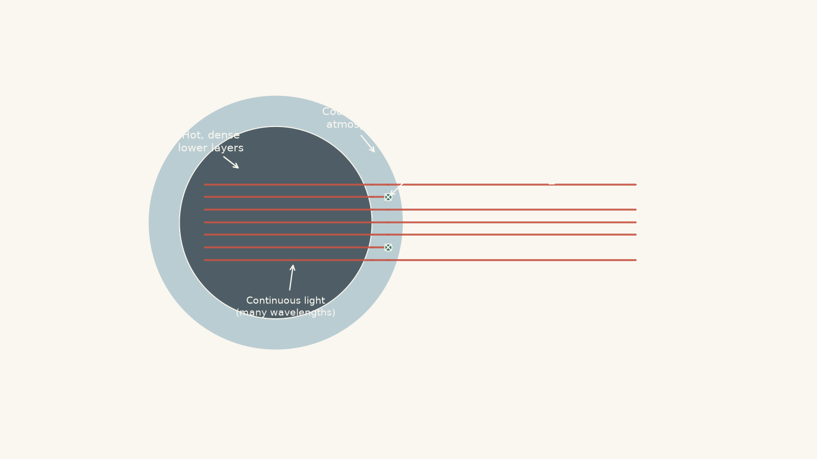
Atoms can absorb only photons with certain energies. Those photon energies correspond to allowed changes between electron energy levels.
A useful first model is an apartment building with some missing floors. An electron is allowed to live on floor 1, 2, 3, and so on, but it cannot stop halfway between them. A photon can make the electron jump upwards only if it delivers exactly the required amount of energy. Turn up with the wrong amount and, rather rudely, the atom ignores you.
The analogy has a limit. Atomic energy levels are quantum states, not physical floors, and whether absorption occurs also depends on probabilities associated with each transition. But the central idea is correct: only particular photon energies can be absorbed.
The energy of a photon is
\[
E = hf = \frac{hc}{\lambda}
\]
where:
- \(E\) is the photon energy in joules, J,
- \(h = 6.63 \times 10^{-34}\ \text{J s}\) is Planck’s constant,
- \(f\) is the frequency in hertz, Hz,
- \(c = 3.00 \times 10^8\ \text{m s}^{-1}\) is the speed of light, and
- \(\lambda\) is the wavelength in metres, m.
If an electron moves between two energy levels separated by energy \(\Delta E\), absorption is possible when
\[
\Delta E = hf = \frac{hc}{\lambda}.
\]
The simplified story says that these photons are “removed”. More precisely, absorbed photons may later be re-emitted in different directions, and energy can also be transferred through collisions. From our particular line of sight, however, less light arrives at those wavelengths. We see a dark absorption line.
02Line position reveals composition
Different atoms and ions have different sets of allowed electron energy levels. They therefore absorb different sets of wavelengths.
That makes a group of absorption lines a kind of fingerprint.
One matching line is weak evidence because unrelated species can sometimes have lines at similar wavelengths. Several lines with the correct relative pattern give much stronger evidence.
Suppose laboratory measurements show that an element produces strong absorption lines at 430 nm, 517 nm, and 589 nm. If a stellar spectrum contains lines at all three positions, that pattern is much more convincing than a single match at 589 nm.
This is the basis of identifying elements with spectral lines.
There is an important wording point here. A spectrum normally tells us which atoms or ions are producing detectable absorption in the star’s atmosphere. It does not mean we are directly sampling the entire chemical composition of the whole star.
Worked example: What does a hydrogen absorption line actually tell us?
A stellar spectrum contains absorption lines at 410.2 nm, 434.0 nm, 486.1 nm, and 656.3 nm. These wavelengths match a known group of hydrogen lines. Calculate the photon energy corresponding to the 486.1 nm line, then explain why the group of lines is better evidence for hydrogen than the 486.1 nm line alone.
Step 1
\[
\lambda = 486.1\ \text{nm}
= 486.1 \times 10^{-9}\ \text{m}
= 4.861 \times 10^{-7}\ \text{m}
\]
Step 2
\[
E = \frac{hc}{\lambda}
= \frac{(6.63\times10^{-34})(3.00\times10^8)}
{4.861\times10^{-7}}
= 4.09\times10^{-19}\ \text{J}
\]
So the absorbing hydrogen atom takes up a photon carrying approximately
\[
E = 4.09\times10^{-19}\ \text{J}.
\]
That energy corresponds to a particular allowed electron transition.
Step 3
A single line at 486.1 nm would not uniquely prove that hydrogen was responsible. The additional matches at 410.2 nm, 434.0 nm, and 656.3 nm make the identification much stronger because the whole pattern agrees with hydrogen.
The result tells us that hydrogen capable of producing these transitions is present in the absorbing atmosphere. It does not yet tell us exactly how much hydrogen the star contains.
03Why a darker line does not simply mean “more of that element”
Imagine two stars. Star A has a very dark hydrogen line. Star B has a much weaker version of the same line.
Which star contains more hydrogen?
You cannot safely tell from that information alone.
For an atom to absorb a particular photon, it must already be in the correct starting energy state. Temperature changes how many atoms occupy each energy level. At still higher temperatures, collisions can remove electrons completely, producing ions.
This means absorption-line strength depends on several things, including:
- how much of the element is present,
- the star’s atmospheric temperature,
- how strongly that particular atomic transition interacts with light,
- what fraction of the atoms are ionised,
- what fraction of the atoms have electrons in the required starting energy level, and
- the pressure and density of the atmosphere.
Hydrogen gives a classic example. Its visible Balmer absorption lines require electrons to begin in the \(n=2\) energy level.
In a relatively cool stellar atmosphere, many hydrogen atoms exist, but comparatively few have electrons in \(n=2\). The Balmer lines can therefore be weak.
Raise the temperature and more hydrogen atoms occupy excited states, so the Balmer lines become stronger.
Raise the temperature much further and a larger proportion of the hydrogen becomes ionised. An ionised hydrogen atom has lost its electron, so it cannot make the same Balmer absorption transition. The lines can weaken again.
So the hottest star does not necessarily have the strongest hydrogen absorption lines, and the star with the strongest hydrogen lines does not necessarily contain the most hydrogen.
That is why composition and temperature have to be interpreted together. The connection is explored further in finding stellar temperature from spectra.
04Line width gives a different clue
So far, we have mainly cared about where a line appears and how strongly it absorbs. Its width also contains information.
An absorption line is not perfectly thin. Instead, it has a profile spread across a small wavelength range.
One reason is collisions.
Atoms and charged particles in a stellar atmosphere constantly interact. In a higher-pressure, higher-density gas, those interactions happen more frequently. Collisions and nearby electric fields disturb the atomic energy states slightly, meaning absorption occurs across a range of very similar photon energies rather than at one infinitely precise energy.
The result is pressure broadening: absorption lines become wider.
For hydrogen in hot stellar atmospheres, interactions with surrounding charged particles can produce particularly important broadening known as Stark broadening.
The useful HSC-level chain is
\[
\text{higher atmospheric density}
\rightarrow \text{more interactions}
\rightarrow \text{greater pressure broadening}
\rightarrow \text{wider spectral lines}.
\]
But there is a condition attached to that conclusion. Other effects can broaden lines too.
These include:
- thermal motion of particles,
- rotation of the star,
- large-scale gas motion, and
- the limited resolution of the spectrometer.
So “wide line = dense star” is not a complete rule.
What we can say is that, after other broadening mechanisms have been accounted for, stronger pressure broadening can provide evidence of greater pressure and particle density in the line-forming region of the stellar atmosphere.
It does not directly give the average density of the entire star.
Worked example: Which atmosphere is denser?
Two stars have the same atmospheric temperature and similar chemical composition. Rotational and instrumental broadening have already been corrected for. The same absorption line is centred at 500.0 nm in both stars.
For Star P, the line width is 0.14 nm. For Star Q, it is 0.42 nm.
Assuming pressure broadening is the important remaining difference, which star has the higher atmospheric pressure and density?
Step 1
\[
\frac{\Delta\lambda_Q}{\Delta\lambda_P}
=
\frac{0.42}{0.14}
= 3.0
\]
Star Q’s line is three times as wide.
Step 2
The problem tells us that temperature, composition, rotation, and instrumental effects are controlled. The remaining broadening is therefore being attributed to pressure effects.
More frequent interactions in the denser gas disturb the relevant atomic energy states more strongly.
Step 3
Star Q has the higher atmospheric pressure and particle density in the region producing the line.
The factor of three in line width does not mean the density is exactly three times greater. The relationship between pressure, density, and detailed line shape requires an atmospheric model and depends on the transition involved.
That distinction matters: a spectrum can support a comparison of atmospheric densities without giving a simple one-step conversion from nanometres to kilograms per cubic metre.
05Surface gravity helps explain the density difference
Why might two stars with similar temperatures have different atmospheric pressures in the first place?
Gravity matters.
Near the surface of a roughly spherical star,
\[
g = \frac{GM}{R^2}
\]
where:
- \(g\) is the surface gravitational field strength in \(\text{m s}^{-2}\),
- \(G\) is the universal gravitational constant,
- \(M\) is the star’s mass in kilograms, and
- \(R\) is its radius in metres.
A star with stronger surface gravity holds its atmospheric gas more tightly. Under otherwise similar conditions, that tends to produce greater atmospheric pressure in the layers where absorption lines form.
A giant star can therefore have a very large total size while still having a relatively low-pressure outer atmosphere. A smaller star of comparable mass can have stronger surface gravity and more strongly pressure-broadened lines.
This is a nice trap because “bigger star” sounds as though it should mean “more stuff packed into the atmosphere”. Radius by itself does not decide the surface conditions. Gravity depends on both mass and \(R^2\).

06Read an absorption spectrum as three separate clues
A useful exam habit is to split the evidence before making a conclusion.
| Feature of the absorption line | Main information it can provide | What it does not prove by itself |
|---|---|---|
| Wavelength or pattern of line positions | Identity of atoms or ions | Their exact abundance |
| Line strength or depth | How strongly that transition is absorbing under those atmospheric conditions | That a darker line automatically means more of the element |
| Line width and shape | Pressure, density, thermal motion, rotation, or other broadening processes | Atmospheric density unless competing broadening mechanisms are considered |
| Common shift of an entire line pattern | Motion along the line of sight may be affecting the spectrum | That the element identity has changed |
This prevents one observation from being asked to do too much work.
07The most tempting misconception: “No line means no element”
Suppose an astronomer looks for a particular neutral helium line and cannot see it.
It is tempting to conclude that helium is absent.
That conclusion is too strong.
The atmosphere might be at the wrong temperature for many helium atoms to occupy the required starting state. The helium might instead be strongly ionised. The relevant line might be weak compared with the continuum, blended with another feature, or below the instrument’s detection limit.
A detected pattern can be strong positive evidence that a species is present. A missing line is usually harder to interpret.
This asymmetry is worth remembering:
- matching several predicted lines can identify an element or ion,
- the strength of those lines helps only when temperature and atmospheric conditions are considered, and
- the absence of one expected line does not automatically establish absence of the element.
08Questions and solutions
Question 1
A laboratory spectrum of element X contains strong absorption lines at 448 nm, 502 nm, and 617 nm. A star shows absorption lines at the same three wavelengths.
What is the strongest conclusion supported by this evidence, and why is it better to use all three lines rather than only the 502 nm line?
Solution 1
Element X is present in the line-forming region of the star’s atmosphere, assuming the observed pattern is not produced by coincident overlapping lines from other species.
Each absorption wavelength corresponds to an allowed transition between energy levels in atoms or ions of element X. Matching all three laboratory wavelengths provides a characteristic pattern.
A tempting route is to say that one 502 nm line proves the presence of X. That is weaker reasoning because another species could have a transition near the same wavelength. Several matching lines make an accidental match much less plausible.
The spectrum identifies the absorbing species. It does not, from these wavelengths alone, tell us how abundant element X is.
Question 2
Star A and Star B have the same overall hydrogen abundance. Star A has an atmospheric temperature near 9,500 K, while Star B is much hotter and has a large fraction of its hydrogen ionised.
Star A shows much stronger visible hydrogen absorption lines.
A student concludes that the stronger lines prove Star A contains more hydrogen. Explain why the conclusion is incorrect.
Solution 2
The stronger hydrogen lines in Star A do not prove that Star A contains more hydrogen; the difference can be produced by the different atomic states of hydrogen at the two temperatures.
Visible Balmer absorption requires a hydrogen atom to have an electron in the \(n=2\) state before it absorbs the photon.
At an appropriate intermediate temperature, enough hydrogen atoms occupy that starting state for strong Balmer absorption to occur. In the much hotter atmosphere of Star B, a larger fraction of hydrogen is ionised. Once hydrogen has lost its electron, that atom cannot produce the same Balmer absorption transition.
The tempting argument is
\[
\text{stronger line} \rightarrow \text{more hydrogen}.
\]
The missing step is the fraction of hydrogen atoms actually capable of making that transition. Line strength depends on abundance and physical conditions.
The correct interpretation is that Star A has more hydrogen atoms in the states required to produce strong Balmer absorption, not necessarily more total hydrogen.
Question 3
An absorption line is observed at \(486.1\ \text{nm}\).
Calculate the energy of one photon removed at this wavelength. An atomic species in the stellar atmosphere has an allowed energy difference of \(4.09\times10^{-19}\ \text{J}\). Explain what the calculation tells you, and what further evidence you would want before confidently identifying the species.
Use \(h=6.63\times10^{-34}\ \text{J s}\) and \(c=3.00\times10^8\ \text{m s}^{-1}\).
Solution 3
The photon energy is \(4.09\times10^{-19}\ \text{J}\), so the observed wavelength is energetically consistent with the stated atomic transition, but one matching line is not enough for a confident identification.
First convert the wavelength:
\[
\lambda
=486.1\ \text{nm}
=4.861\times10^{-7}\ \text{m}.
\]
Then
\[
E=\frac{hc}{\lambda}
=
\frac{(6.63\times10^{-34})(3.00\times10^8)}
{4.861\times10^{-7}}
=
4.09\times10^{-19}\ \text{J}.
\]
This agrees with the stated energy difference.
The physical meaning is that a photon at 486.1 nm carries exactly the energy required for that allowed electron transition.
The tempting conclusion is therefore, “The species must be present.” The problem is that another species might have a line at a nearby wavelength, and measurement uncertainties or Doppler shifts may also affect the observed position.
A stronger identification would use several absorption lines from the same species and check that their overall wavelength pattern agrees with laboratory measurements.
Question 4
Two stars have the same mass, approximately the same atmospheric temperature, and the same chemical composition. Star G has a radius five times larger than Star D.
Assume rotational broadening is negligible.
- Calculate the ratio \(g_G/g_D\) of their surface gravitational field strengths.
- Predict which star should generally have the lower-pressure outer atmosphere.
- Predict which star should show narrower pressure-broadened absorption lines, and explain the complete chain of reasoning.
Solution 4
Star G has only \(1/25\) of Star D’s surface gravitational field strength, so Star G should generally have the lower-pressure outer atmosphere and narrower pressure-broadened spectral lines.
For the same stellar mass,
\[
g=\frac{GM}{R^2}.
\]
Since
\[
R_G=5R_D,
\]
the gravity ratio is
\[
\frac{g_G}{g_D}
=
\frac{GM/(5R_D)^2}{GM/R_D^2}
=
\frac{1}{25}.
\]
So
\[
g_G=0.04g_D.
\]
The larger star therefore has much weaker surface gravity.
With weaker gravity, its outer atmospheric gas is held less tightly. Under the assumptions in the question, this leads to lower pressure and lower particle density in the relevant line-forming layers.
Lower particle density means fewer interactions that disturb atomic energy states. Pressure broadening is therefore reduced, giving narrower absorption lines.
The tempting prediction is that the much larger star should have the denser atmosphere because it is physically bigger. The relevant constraint is not the star’s size by itself. Surface gravity depends on \(M/R^2\).
The complete chain is
\[
R_G \uparrow
\rightarrow g_G \downarrow
\rightarrow \text{atmospheric pressure and density} \downarrow
\rightarrow \text{collisional broadening} \downarrow
\rightarrow \text{narrower lines}.
\]
This conclusion concerns the outer atmosphere producing the spectrum. It is not a direct comparison of the stars’ average internal densities.
Question 5
A rapidly rotating star has two absorption lines centred at 400.0 nm and 600.0 nm. Their measured widths are 0.20 nm and 0.30 nm respectively.
A student notices that both lines are quite broad and concludes that the star must have an unusually dense atmosphere.
For motion at speeds much less than \(c\), Doppler broadening caused by rotation should produce approximately the same fractional wavelength width,
\[
\frac{\Delta\lambda}{\lambda},
\]
for different lines.
- Calculate \(\Delta\lambda/\lambda\) for each observed line.
- Determine the characteristic speed corresponding to that fractional Doppler width using
\[
\frac{\Delta\lambda}{\lambda}\approx\frac{v}{c}.
\]
- The centres of both lines remain at their normal laboratory wavelengths. Explain why this does not rule out rotational Doppler broadening.
- Decide whether the broad lines, by themselves, justify the conclusion that the stellar atmosphere has unusually high density.
Use \(c=3.00\times10^8\ \text{m s}^{-1}\).
Solution 5
The two lines have the same fractional width, \(5.0\times10^{-4}\), corresponding to a characteristic Doppler speed of about \(1.5\times10^5\ \text{m s}^{-1}\), or \(150\ \text{km s}^{-1}\). The pattern is therefore consistent with rotational Doppler broadening, and the broad lines alone do not establish unusually high atmospheric density.
For the 400.0 nm line,
\[
\frac{\Delta\lambda}{\lambda}
=
\frac{0.20}{400.0}
=
5.0\times10^{-4}.
\]
For the 600.0 nm line,
\[
\frac{\Delta\lambda}{\lambda}
=
\frac{0.30}{600.0}
=
5.0\times10^{-4}.
\]
Both lines therefore have the same fractional width.
Using the approximate Doppler relation,
\[
\frac{\Delta\lambda}{\lambda}
\approx
\frac{v}{c},
\]
we obtain
\[
v
\approx
c\frac{\Delta\lambda}{\lambda}
=
(3.00\times10^8)(5.0\times10^{-4})
=
1.5\times10^5\ \text{m s}^{-1}.
\]
So the characteristic speed is
\[
v\approx150\ \text{km s}^{-1}.
\]
The surprising part is that rotation can broaden a line without moving its centre.
One edge of the rotating star is moving towards us, so absorption from that region is blueshifted. The opposite edge is moving away, so its absorption is redshifted. Light from the unresolved stellar disc contains contributions from many different line-of-sight velocities.
The redshifted and blueshifted contributions spread the absorption across a wider wavelength range, but they are approximately symmetric. Their effects on the central wavelength can cancel even while the line becomes much broader.
The tempting reasoning is
\[
\text{broad line}
\rightarrow
\text{pressure broadening}
\rightarrow
\text{high density}.
\]
The missing step is checking for competing broadening mechanisms. Here, the equal fractional widths are exactly the behaviour expected from a Doppler mechanism associated with rotation.
The spectrum therefore does not justify claiming high atmospheric density from line width alone. Density could still contribute to the line shape, but it would have to be separated from rotation, thermal motion, and instrumental effects before making that inference.
Once you can separate line position, line strength, and line width, a stellar spectrum becomes much more useful. Position can identify absorbing species, strength must be interpreted alongside temperature and ionisation, and width can reveal atmospheric conditions only after other broadening mechanisms are considered. The next step is using shifts and broadening caused by motion to extract stellar velocities rather than mistaking motion for a change in composition or density.