
HSC Physics Graphs: How to Use Gradient and Area
A practical guide for HSC Physics students to interpret mechanics and electricity graphs. Learn how to choose between gradient and area, apply the ideas, and avoid common graph mistakes.
A graph can look easy and still hide the physics. A straight line might be showing constant acceleration, a changing force, or simply a relationship that has no useful physical meaning unless you know what the axes represent.
Imagine you are given a velocity-time graph in an exam. The line slopes upwards. What should you say? Many students immediately think “the object is moving faster”, which is true, but it is not enough. The gradient tells you the acceleration. The area under the graph tells you displacement. Two different features of the same picture reveal two different parts of the motion.
The decision you need this reference for is:
- Need to know how quickly one quantity changes? Find the gradient.
- Need to know how much of something has accumulated over time or distance? Find the area.
- Need to know whether a graph represents a real physical relationship? Check the axes, units, and conditions first.
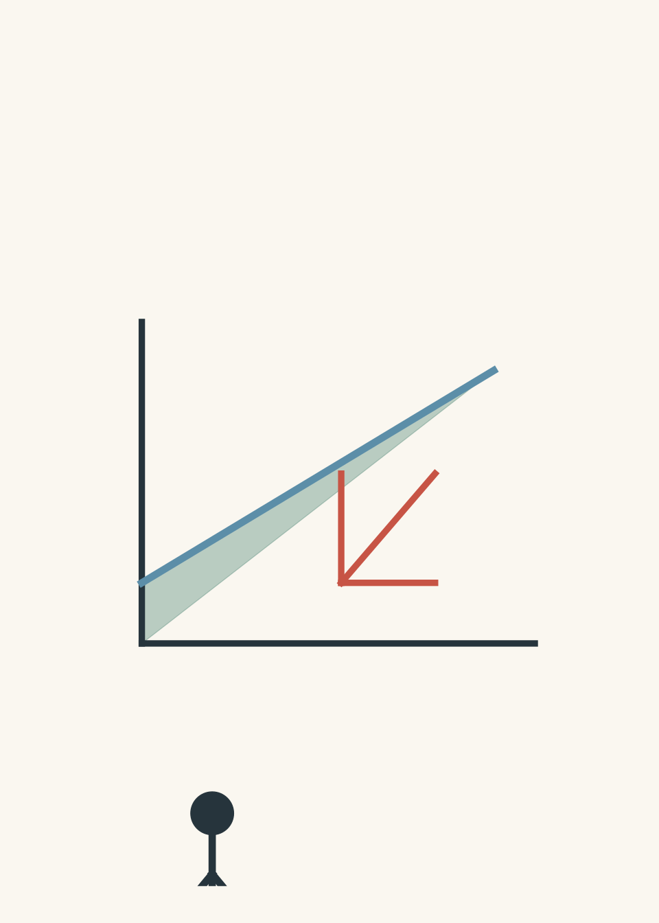
01The first question: what do the axes represent?
Before calculating anything, ignore the shape of the graph for a moment.
A graph is a relationship between two measured quantities. The x-axis is usually the independent variable, and the y-axis is the dependent variable.
For example:
- A velocity-time graph shows how velocity changes as time passes.
- A force-distance graph shows how force changes as an object moves.
- A potential difference-current graph shows how electrical current changes when voltage changes.
The same mathematical feature can mean different physics depending on the axes.
A slope of \(5\) on a graph of distance against time means something different from a slope of \(5\) on a graph of velocity against time.
So the first habit is:
- Read the x-axis and y-axis labels.
- Check the units.
- Ask what physical quantity the gradient or area would produce.
02A quick decision rule for HSC graph problems
| Graph type | Gradient represents | Area represents |
|---|---|---|
| Displacement-time | Velocity | Usually no standard HSC meaning |
| Velocity-time | Acceleration | Displacement |
| Acceleration-time | Rate of change of acceleration (rarely useful directly) | Change in velocity |
| Force-distance | Not usually a key quantity | Work done |
| Voltage-current | Resistance if \(V\) is plotted against \(I\) | Usually not used |
| Current-time | Not usually used | Charge transferred |
The table only applies when the graph axes are arranged as shown. Swapping the axes changes the meaning.
For example, a voltage-current graph and a current-voltage graph are not interchangeable. The gradient changes from resistance to reciprocal resistance.
03Gradient: the physics of “how fast something changes”
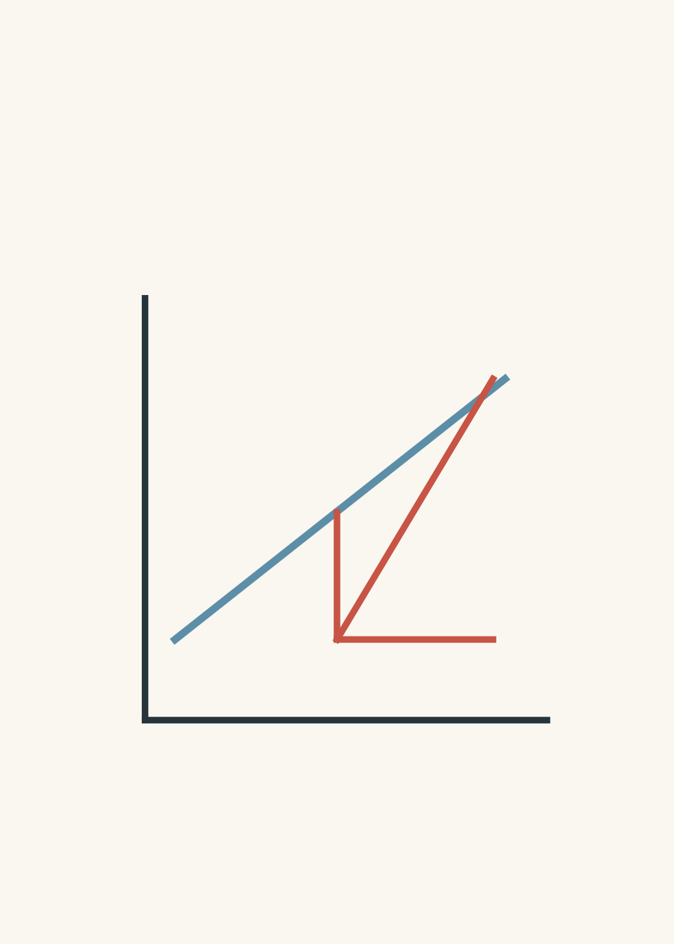
A gradient is calculated using:
\[
\text{gradient} = \frac{\text{change in vertical quantity}}{\text{change in horizontal quantity}}
\]
or:
\[
m = \frac{\Delta y}{\Delta x}
\]
where:
- \(m\) is the gradient,
- \(\Delta y\) is the change in the y-axis quantity,
- \(\Delta x\) is the change in the x-axis quantity.
The units of the gradient come from the units of the axes.
For example, on a velocity-time graph:
\[
\frac{\text{m/s}}{\text{s}} = \text{m/s}^2
\]
which is acceleration.
Why gradient works
Think about walking down a path.
If you travel 100 m in 20 s, your average speed is:
\[
\frac{100\text{ m}}{20\text{ s}} = 5\text{ m/s}
\]
You are comparing how much distance changed with how much time changed.
A graph gradient does the same thing. It compares the change in one quantity with the change in another.
A useful analogy is a relationship where one person is constantly changing how much attention they give another person. The “gradient” is like asking, “How quickly is this changing?” A steep change means the situation is changing rapidly. A flat line means no change.
The analogy breaks down because physical graphs have precise units and measurements. A gradient is not just “more” or “less”; it has a defined meaning.
04The gradient of common HSC physics graphs
Displacement-time graphs
Velocity is the rate of change of displacement.
\[
v = \frac{\Delta x}{\Delta t}
\]
where:
- \(v\) is velocity in m/s,
- \(\Delta x\) is change in displacement in m,
- \(\Delta t\) is change in time in s.
A straight line means constant velocity.
A curved line means the velocity is changing.
A common mistake is to say that a steeper displacement-time graph means “more acceleration”. It does not. A steeper graph means a larger velocity.
Acceleration only appears when velocity changes.
Velocity-time graphs
The gradient gives acceleration.
\[
a = \frac{\Delta v}{\Delta t}
\]
where:
- \(a\) is acceleration in m/s²,
- \(\Delta v\) is change in velocity in m/s,
- \(\Delta t\) is change in time in s.
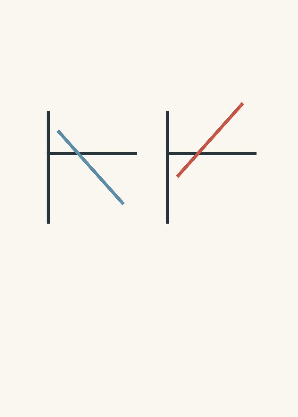
A positive gradient means positive acceleration.
A negative gradient means negative acceleration.
However, negative acceleration does not always mean slowing down. If an object is already moving in the negative direction, negative acceleration can make it speed up.
05Area: the physics of accumulation
Area under a graph is found using:
\[
\text{area} = \text{base} \times \text{height}
\]
for simple rectangles and triangles.
The units multiply together.
For a velocity-time graph:
\[
(\text{m/s}) \times (\text{s}) = \text{m}
\]
so the area represents displacement.
For a force-distance graph:
\[
(\text{N}) \times (\text{m}) = \text{J}
\]
so the area represents work done.
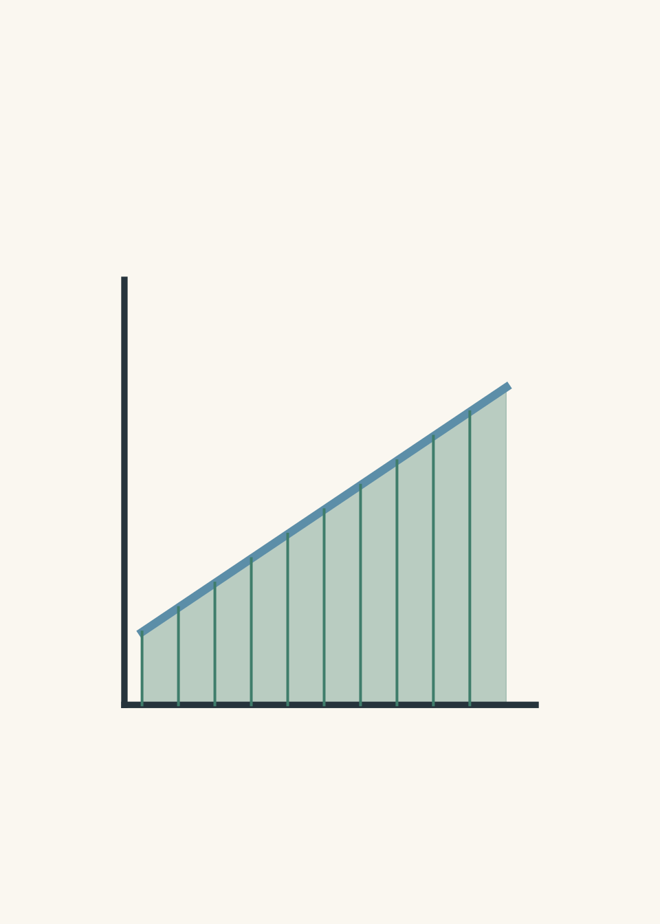
The important idea is that area adds up many small changes.
Imagine tracking your location every second. Each tiny strip of a velocity-time graph represents a small displacement during that second. Adding all the strips gives total displacement.
06Worked example: finding acceleration from a velocity-time graph
A car increases its velocity from \(4.0\text{ m/s}\) to \(16.0\text{ m/s}\) over \(6.0\text{ s}\). Find its acceleration.
Step 1
The question asks how quickly velocity changes, so use the gradient of a velocity-time graph.
Step 2
\[
a = \frac{\Delta v}{\Delta t}
\]
Step 3
\[
a = \frac{16.0 – 4.0}{6.0}
\]
\[
a = \frac{12.0}{6.0}
\]
\[
a = 2.0\text{ m/s}^2
\]
Step 4
The acceleration is \(2.0\text{ m/s}^2\). The car’s velocity increases by \(2.0\text{ m/s}\) every second.
The trap is using the final velocity instead of the change in velocity. Gradient always uses the difference between two points.
07Worked example: finding displacement from a velocity-time graph
A cyclist moves with a constant velocity of \(8.0\text{ m/s}\) for \(15\text{ s}\). Find the displacement.
Step 1
A velocity-time graph gives displacement through its area.
The graph is a rectangle because velocity is constant.
Step 2
\[
\text{displacement} = \text{velocity} \times \text{time}
\]
Step 3
\[
\text{displacement} = 8.0 \times 15
\]
\[
\text{displacement} = 120\text{ m}
\]
Step 4
The cyclist moves \(120\text{ m}\) in the direction of the velocity.
The common trap is looking for the gradient because gradients feel like the “physics part” of graphs. In this situation, the area is the useful feature.
08Electricity graphs: the same ideas in a different setting
Graphs are not only about motion.
In electricity, the axes decide the meaning.
For an ohmic conductor:
\[
V = IR
\]
where:
- \(V\) is potential difference in volts,
- \(I\) is current in amperes,
- \(R\) is resistance in ohms.
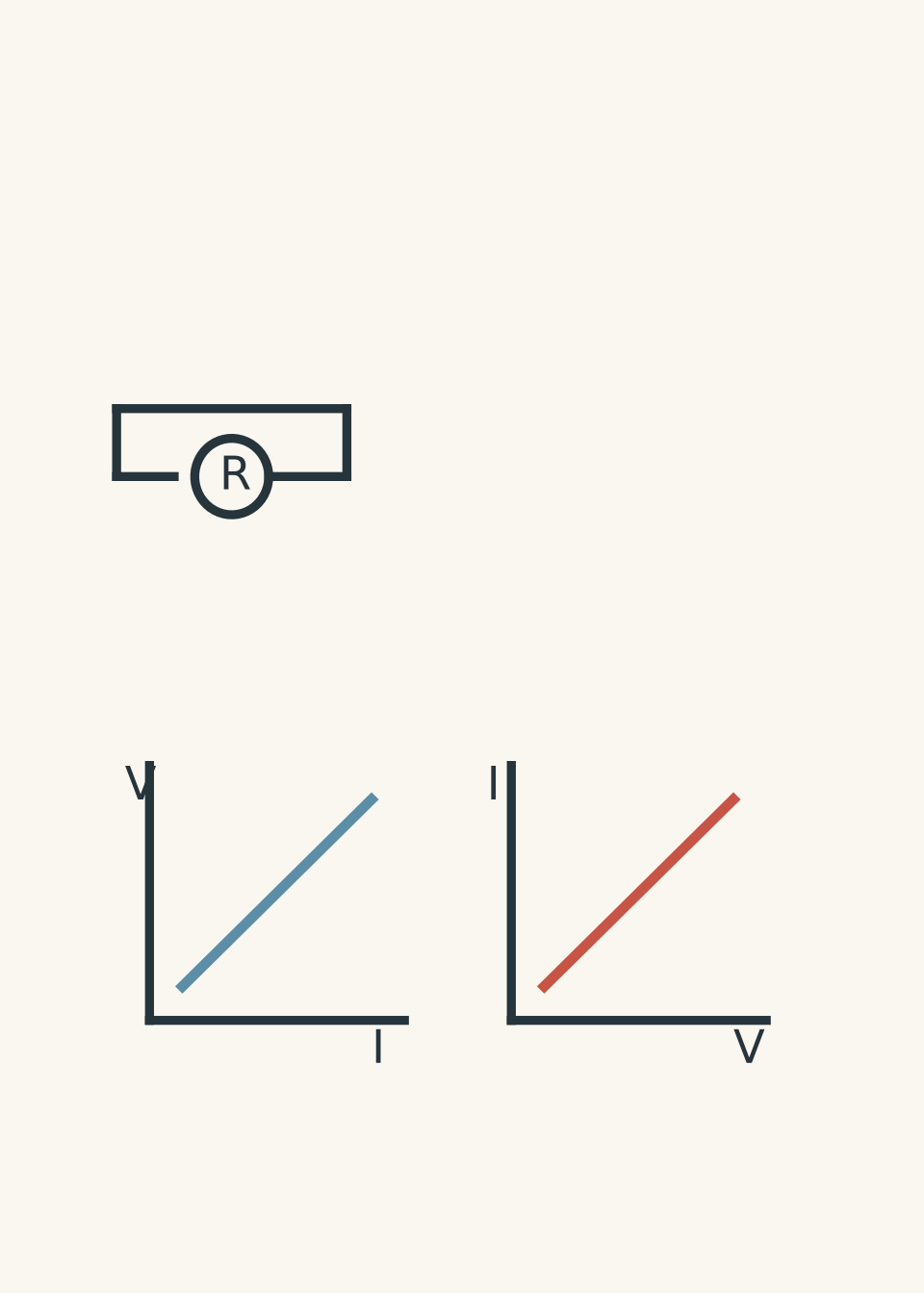
If a graph plots voltage on the y-axis and current on the x-axis:
\[
\text{gradient} = \frac{V}{I} = R
\]
The gradient gives resistance.
If the graph is current on the y-axis and voltage on the x-axis:
\[
\text{gradient} = \frac{I}{V} = \frac{1}{R}
\]
The same data can produce a different gradient meaning because the axes have changed.
09When the simple model fails
Graphs often begin with ideal situations.
A straight velocity-time line assumes constant acceleration.
A straight voltage-current line assumes constant resistance.
Real systems often change.
For example, a filament lamp does not behave like an ohmic conductor because its resistance changes as the filament heats up. The graph curves because the relationship changes.
The skill is not memorising “straight line equals this”. The skill is asking:
“What physical condition would need to stay constant for this graph shape to occur?”
10Common mistakes
Reading the graph shape before reading the axes
A student sees a steep line and assumes it means acceleration.
The fix: identify the quantities first. A steep line only means a large rate of change between the chosen axes.
Confusing velocity with acceleration
A velocity-time graph that slopes upwards shows acceleration. A velocity-time graph that is horizontal still shows motion, but the acceleration is zero.
Using area when the units do not match
Area only gives a useful physical quantity if multiplying the axes produces meaningful units.
For example:
\[
(\text{m/s}) \times (\text{s}) = \text{m}
\]
works for displacement.
Forgetting negative areas
On a velocity-time graph, areas below the time axis represent displacement in the opposite direction.
The area is not always total distance travelled.
Assuming a graph must be linear
A curved graph often contains more information, not less. The changing gradient can show changing acceleration, resistance, or another changing physical property.
11Questions and solutions
Question 1
A train’s velocity increases from \(10\text{ m/s}\) to \(22\text{ m/s}\) in \(4.0\text{ s}\).
Calculate the acceleration.
Solution 1
The acceleration is \(3.0\text{ m/s}^2\). The gradient of a velocity-time graph gives acceleration because it measures the change in velocity per unit time.
\[
a=\frac{\Delta v}{\Delta t}
\]
\[
a=\frac{22-10}{4.0}
\]
\[
a=\frac{12}{4.0}
\]
\[
a=3.0\text{ m/s}^2
\]
A tempting mistake is to use \(22/4.0\), but that assumes the train started from rest. The graph tells us the velocity changed from \(10\text{ m/s}\), not \(0\text{ m/s}\).
Question 2
A velocity-time graph shows an object moving at \(6.0\text{ m/s}\) for \(5.0\text{ s}\), then slowing uniformly to \(0\text{ m/s}\) over the next \(3.0\text{ s}\).
Find the total displacement.
Solution 2
The total displacement is \(39\text{ m}\). The area under the velocity-time graph must be separated into two regions.
First section:
\[
\text{area}=6.0 \times 5.0=30\text{ m}
\]
Second section is a triangle:
\[
\text{area}=\frac{1}{2}\times3.0\times6.0
\]
\[
\text{area}=9.0\text{ m}
\]
Total displacement:
\[
30+9=39\text{ m}
\]
The tempting route is to use average velocity over the whole 8 seconds. That only works if you correctly account for the changing velocity. The area method works directly because each section of the graph represents displacement.
Question 3
A student claims:
“A negative gradient on a velocity-time graph always means the object is slowing down.”
Explain whether this statement is correct.
Solution 3
The statement is incorrect. A negative gradient means the acceleration is negative, but the object may either slow down or speed up depending on its velocity direction.
For an object moving with positive velocity, a negative acceleration reduces its speed.
For an object already moving with negative velocity, a negative acceleration makes the velocity more negative, increasing its speed.
The trap is confusing acceleration direction with speed change. Acceleration tells you how velocity changes, not whether the speed increases or decreases.
Question 4
A resistor is tested by measuring voltage and current. A graph of voltage on the y-axis against current on the x-axis gives a straight line with a gradient of \(12\text{ V/A}\).
The same data is replotted with current on the y-axis and voltage on the x-axis.
What is the new gradient, and what does it represent?
Solution 4
The new gradient is \(0.083\text{ A/V}\), which represents the reciprocal of resistance, or conductance.
From the first graph:
\[
R=\frac{V}{I}=12\Omega
\]
The second graph has gradient:
\[
\frac{I}{V}=\frac{1}{R}
\]
\[
\frac{1}{12}=0.083\text{ A/V}
\]
The tempting mistake is to keep the value \(12\) because the physical data has not changed. The constraint that changes the answer is the axis order. Gradient depends on what is plotted vertically and horizontally.
Question 5
An object moves along a straight path. Its velocity-time graph is a straight line from \(t=0\) to \(t=10\text{ s}\). The graph starts at \(v=-4.0\text{ m/s}\) and ends at \(v=6.0\text{ m/s}\).
A student says:
“The object must have travelled \(60\text{ m}\) because its final velocity is \(6.0\text{ m/s}\) and the motion lasted \(10\text{ s}\).”
Determine the displacement and explain why the student’s reasoning fails.
Solution 5
The displacement is \(10\text{ m}\), not \(60\text{ m}\). The student’s reasoning fails because the velocity was not constant and because the object initially moved in the opposite direction.
The displacement is the signed area under the velocity-time graph.
The line crosses \(v=0\) halfway through because the velocity changes uniformly from \(-4.0\text{ m/s}\) to \(6.0\text{ m/s}\).
The negative triangle:
\[
\text{area}=-\frac{1}{2}\times4.0\times4.0=-8.0\text{ m}
\]
The positive triangle:
\[
\text{area}=\frac{1}{2}\times6.0\times6.0=18\text{ m}
\]
Total displacement:
\[
18-8=10\text{ m}
\]
The tempting route is to multiply final velocity by total time. That would only be valid if the velocity stayed at \(6.0\text{ m/s}\) for the entire interval. The deeper idea is that a velocity-time graph records the whole history of the motion, not just the final state.
12Next step: using graphs to test equations
Once you can read gradients and areas, the next useful skill is recognising the equation hidden inside a graph.
A straight-line graph is often a physical law written visually:
\[
y=mx+c
\]
The gradient tells you the relationship between variables, and the intercept can reveal an initial value or a physical constant. In HSC Physics, this is where graphs become more than pictures: they become tools for testing models.