
Calorimetry Heat Loss: Why Exothermic ΔH Looks Less Negative
Learn how heat escaping from a calorimeter affects the measured temperature change and makes an exothermic enthalpy change appear less negative. Includes worked calculations, practical experimental improvements, and HSC-style questions with detailed solutions.
Mix 50.0 mL of 1.00 mol L\\(^{-1}\\) hydrochloric acid, \\(\ce{HCl}\\), with 50.0 mL of 1.00 mol L\\(^{-1}\\) sodium hydroxide, \\(\ce{NaOH}\\). The solution warms from 21.00°C to 27.00°C, giving an experimental enthalpy of about \\(-50.2\ \mathrm{kJ\,mol^{-1}}\\), even though strong acid-strong base neutralisation is usually around \\(-57\ \mathrm{kJ\,mol^{-1}}\\).
Has the reaction released less energy than it should? Before blaming the chemistry, predict what happens if some of the released heat warms the cup and surrounding air instead of the solution being measured.
01The experiment measures temperature, not heat directly
A common way to measure enthalpy changes in the school laboratory is to use a coffee-cup calorimeter. The apparatus is simple, but understanding what it measures – and what it misses – is the key to getting the correct result.

The experiment follows a straightforward sequence:
- Measure the initial temperatures of the reactant solutions.
- Mix the reactants in the insulated cup.
- Replace the lid, stir the mixture, and record the temperature as the reaction proceeds.
- Use the temperature change to estimate the heat released by the reaction.
The problem is that the thermometer measures the temperature of the solution, not the total energy released by the reaction.
Some of that energy warms the solution. Some warms the cup, and some escapes into the surrounding air or bench. The basic calculation usually counts only the energy absorbed by the solution.
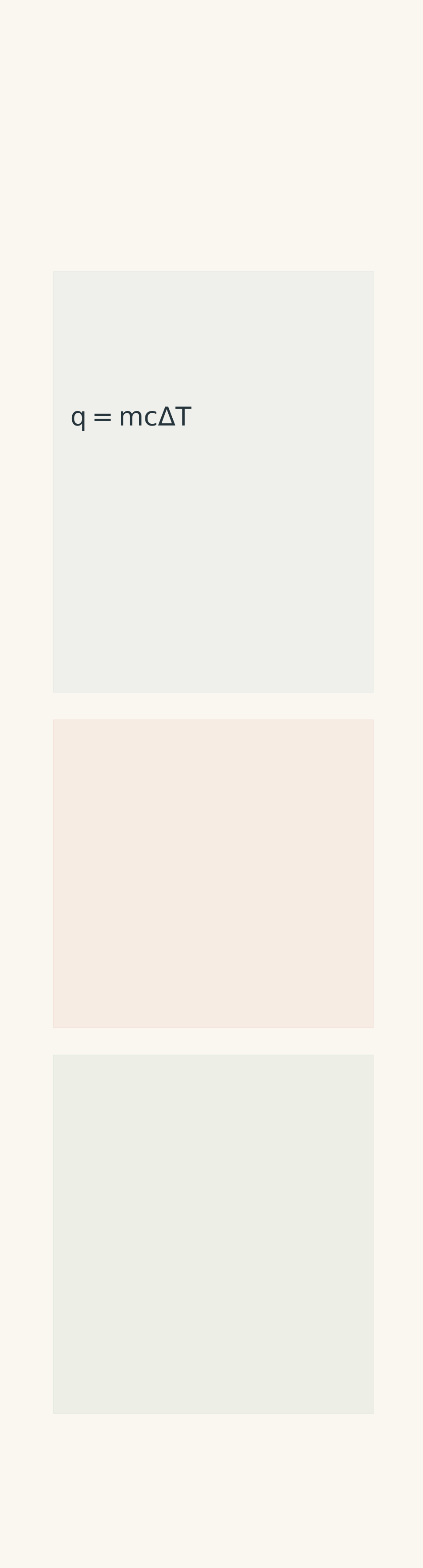
Imagine the released heat as a pizza shared between the solution, the cup, and the room. If you count only the slice eaten by the solution, you underestimate the size of the whole pizza. The analogy is about energy accounting: heat is energy transferred between objects, not a substance that gets divided into literal pieces.
Now return to the opening experiment. If less heat stays in the solution, its temperature rise is smaller. Because the calculated heat depends on that temperature rise, the calculated enthalpy becomes less negative.
02Follow the error through the calculation
Three relationships explain the entire problem.
1. Calculate the heat absorbed by the solution
For a dilute aqueous solution, the heat absorbed is estimated using
\\[ q_{\text{solution}}=mc\Delta T \\]
where:
- \\(q_{\text{solution}}\\) is the heat absorbed by the solution, in joules (J).
- \\(m\\) is the mass of the solution, in grams (g).
- \\(c\\) is the specific heat capacity, usually approximated as \\(4.18\ \mathrm{J\,g^{-1}\,^\circ C^{-1}}\\) for a dilute aqueous solution.
- \\(\Delta T=T_{\text{final}}-T_{\text{initial}}\\) is the temperature change in degrees Celsius.
For an exothermic reaction, the solution warms, so \\(\Delta T\\) and \\(q_{\text{solution}}\\) are positive.
If heat escapes before it can warm the solution, the measured \\(\Delta T\\) is smaller than it would be in an ideal insulated experiment. With \\(m\\) and \\(c\\) unchanged, the calculated \\(q_{\text{solution}}\\) is also smaller.
2. Reverse the sign to estimate the reaction heat
The solution gains energy released by the reaction. Their heat transfers therefore have opposite signs.
Under the simplified assumption that the solution absorbs all the released heat,
\\[ q_{\text{reaction}}\approx-q_{\text{solution}} \\]
The minus sign is important. A solution that gains \\(2.51\ \mathrm{kJ}\\) corresponds to a calculated reaction heat of \\(-2.51\ \mathrm{kJ}\\).
But if the solution captures only part of the released energy, this calculation underestimates the magnitude of the reaction heat. The calculated negative value is closer to zero than the true value.
3. Calculate the molar enthalpy change
At constant pressure, the heat transferred by the reaction corresponds to its enthalpy change. The molar enthalpy change is estimated by dividing the reaction heat by the amount of reaction, expressed in moles:
\\[ \Delta H_{\text{reaction}}\approx \frac{q_{\text{reaction}}}{n} \\]
Here, \\(n\\) is the amount of reaction in moles. For the 1:1 neutralisation of \\(\ce{HCl}\\) by \\(\ce{NaOH}\\), it equals the moles of water formed.
Keep the units consistent: use \\(q\\) in kJ and \\(n\\) in mol to obtain \\(\Delta H\\) in \\(\mathrm{kJ\,mol^{-1}}\\).
The error now follows a clear chain:
- Heat escapes, so the measured temperature rise is too small.
- The calculated \\(q_{\text{solution}}\\) is too small.
- The calculated \\(q_{\text{reaction}}\\) is not negative enough.
- The calculated \\(\Delta H\\) is less negative than the true value.
For example, \\(-50.2\ \mathrm{kJ\,mol^{-1}}\\) is less negative than \\(-57.3\ \mathrm{kJ\,mol^{-1}}\\), because \\(-50.2\\) is closer to zero.
The chemistry has not necessarily changed. The experiment has simply failed to account for all the energy transferred.
03Worked example: calculating the enthalpy of neutralisation
A student mixes 50.0 mL of 1.00 mol L\\(^{-1}\\) \\(\ce{HCl}\\) with 50.0 mL of 1.00 mol L\\(^{-1}\\) \\(\ce{NaOH}\\). The temperature rises from 21.00°C to 27.00°C.
Assume the solution density is \\(1.00\ \mathrm{g\,mL^{-1}}\\), its specific heat capacity is \\(4.18\ \mathrm{J\,g^{-1}\,^\circ C^{-1}}\\), and the cup’s heat capacity is negligible. Calculate the experimental molar enthalpy change.
Step 1: Calculate the mass of the solution.
The total volume is
\\[ V=50.0+50.0=100.0\ \mathrm{mL} \\]
Using the assumed density,
\\[ m=100.0\ \mathrm{mL} \times1.00\ \mathrm{g\,mL^{-1}} =100.0\ \mathrm{g} \\]
Step 2: Calculate the temperature change.
\\[ \begin{aligned} \Delta T&=T_{\text{final}}-T_{\text{initial}}\\ &=27.00-21.00\\ &=6.00^\circ\mathrm{C} \end{aligned} \\]
Step 3: Calculate the heat absorbed by the solution.
Substitute into \\(q_{\text{solution}}=mc\Delta T\\):
\\[ \begin{aligned} q_{\text{solution}} &=100.0\times4.18\times6.00\\ &=2508\ \mathrm{J}\\ &=2.508\ \mathrm{kJ} \end{aligned} \\]
The solution gains \\(2.508\ \mathrm{kJ}\\) of energy.
Step 4: Calculate the amount of reaction.
The balanced equation is
\\[ \ce{HCl(aq) + NaOH(aq) -> NaCl(aq) + H2O(l)} \\]
The amount of hydrochloric acid is
\\[ \begin{aligned} n(\ce{HCl}) &=cV\\ &=1.00\times0.0500\\ &=0.0500\ \mathrm{mol} \end{aligned} \\]
The sodium hydroxide is present in the same amount, so \\(0.0500\ \mathrm{mol}\\) of water forms.
Step 5: Calculate the experimental molar enthalpy change.
Using the simplified assumption that the solution captures all the reaction heat,
\\[ q_{\text{reaction, calc}}=-2.508\ \mathrm{kJ} \\]
Therefore,
\\[ \begin{aligned} \Delta H_{\text{exp}} &=\frac{q_{\text{reaction, calc}}}{n}\\ &=\frac{-2.508}{0.0500}\\ &=-50.16\ \mathrm{kJ\,mol^{-1}} \end{aligned} \\]
The experimental result is approximately \\(-50.2\ \mathrm{kJ\,mol^{-1}}\\).
What does the discrepancy mean?
For comparison, a reference neutralisation enthalpy of \\(-57.3\ \mathrm{kJ\,mol^{-1}}\\) would correspond to \\(0.0500\times57.3=2.865\ \mathrm{kJ}\\) released.
The solution calculation accounts for only \\(2.508\ \mathrm{kJ}\\). The difference is
\\[ 2.865-2.508=0.357\ \mathrm{kJ} \\]
If the entire discrepancy were due to heat escaping to the surroundings, approximately \\(0.357\ \mathrm{kJ}\\) would have escaped. In a real experiment, some of the discrepancy may also come from energy absorbed by the cup.
The important result is that the measured temperature rise leads to an enthalpy value that is too close to zero.
04How the experimental design was improved
The first design is simple: mix the reactants in a cup and measure the temperature. Its underlying assumption is that the solution captures nearly all the released heat.
If that assumption held, the temperature rise would give a reliable estimate of the reaction heat, provided the cup’s heat capacity was negligible or accounted for.
In practice, the temperature rises, reaches a maximum, and then falls. Heat can escape while the reaction is occurring, and the thermometer may also take time to respond. By the time the maximum is recorded, some energy may already have left the measured solution.
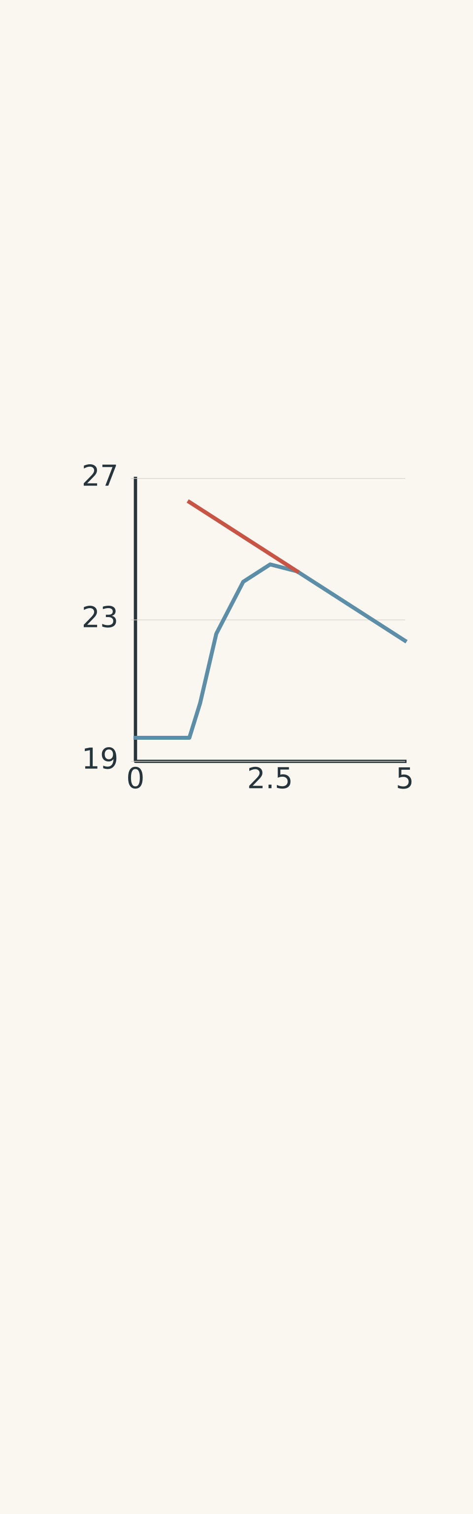
A revised design addresses some of these problems.
- Use two nested polystyrene cups to improve insulation.
- Fit a lid around the thermometer probe and stirrer to reduce heat exchange with the air.
- Stir consistently so the solution has a more uniform temperature.
- Use a temperature probe or data logger to record the temperature throughout the experiment.
- Record the cooling curve after the reaction and, where appropriate, extrapolate it backwards to estimate the temperature before post-reaction cooling.
The last step needs care. If the reaction is rapid compared with the cooling process, extrapolating the cooling segment can estimate how much the solution cooled after the reaction. It does not automatically restore heat that escaped while the reaction was taking place.
The revised apparatus reduces the error, but it does not make the experiment perfectly insulated.
05Worked example: estimating the fraction of heat not captured
A student reacts 25.0 mL of 1.50 mol L\\(^{-1}\\) \\(\ce{HCl}\\) with 25.0 mL of 1.50 mol L\\(^{-1}\\) \\(\ce{NaOH}\\). The total solution mass is 50.0 g, and the temperature rises by 8.00°C.
Using \\(c=4.18\ \mathrm{J\,g^{-1}\,^\circ C^{-1}}\\), calculate the experimental molar enthalpy change. Then estimate the percentage of the reaction heat not captured by the solution, using a reference enthalpy of \\(-57.3\ \mathrm{kJ\,mol^{-1}}\\). Assume the entire discrepancy is due to heat not captured by the solution.
Step 1: Calculate the heat absorbed by the solution.
\\[ \begin{aligned} q_{\text{solution}} &=mc\Delta T\\ &=50.0\times4.18\times8.00\\ &=1672\ \mathrm{J}\\ &=1.672\ \mathrm{kJ} \end{aligned} \\]
Step 2: Calculate the amount of reaction.
The volume of hydrochloric acid is \\(0.0250\ \mathrm{L}\\).
\\[ \begin{aligned} n(\ce{HCl}) &=1.50\times0.0250\\ &=0.0375\ \mathrm{mol} \end{aligned} \\]
The same amount of sodium hydroxide reacts, so \\(0.0375\ \mathrm{mol}\\) of water forms.
Step 3: Calculate the experimental enthalpy change.
\\[ \begin{aligned} \Delta H_{\text{exp}} &=\frac{-1.672}{0.0375}\\ &=-44.6\ \mathrm{kJ\,mol^{-1}} \end{aligned} \\]
The experimental result is less negative than the reference value.
Step 4: Calculate the expected heat released.
Using the magnitude of the reference enthalpy,
\\[ \begin{aligned} Q_{\text{released}} &=n|\Delta H_{\text{reference}}|\\ &=0.0375\times57.3\\ &=2.149\ \mathrm{kJ} \end{aligned} \\]
Step 5: Estimate the heat not captured.
\\[ \begin{aligned} Q_{\text{missed}} &=Q_{\text{released}}-q_{\text{solution}}\\ &=2.149-1.672\\ &=0.477\ \mathrm{kJ} \end{aligned} \\]
Step 6: Calculate the percentage not captured.
\\[ \begin{aligned} \%\text{ missed} &=\frac{0.477}{2.149}\times100\\ &=22.2\% \end{aligned} \\]
Approximately 22.2% of the reference reaction heat was not recorded as energy absorbed by the solution, under the stated assumption. This is an estimate of the experimental shortfall, not proof that exactly that amount entered the surrounding air.
06Systematic heat loss or random measurement variation?
Not every difference between experimental results has the same cause. Distinguishing systematic error from random variation helps you decide what to improve.
Systematic error
A systematic error shifts results in a consistent direction. In an exothermic calorimetry experiment, unaccounted heat loss tends to make the measured temperature rise too small and the calculated enthalpy too close to zero.
Suppose the expected temperature rise is 6.8°C, but repeated trials produce 5.8°C, 5.9°C, and 6.0°C. These results are close together, yet all fall below the expected value.
The experiment is reasonably consistent, but something is biasing the results. Possible causes include heat escaping to the surroundings, heat absorbed by the cup but omitted from the calculation, or a thermometer calibration error.
Random variation
Random variation causes results to scatter. Small differences in stirring, timing, probe response, or reading the maximum temperature may cause individual measurements to be higher or lower.
For example, measurements of 6.4°C, 6.8°C, and 7.2°C are spread around 6.8°C. That pattern is consistent with random variation around the expected value, although three results alone cannot establish its precise statistical nature.

The distinction is useful:
| Pattern in the results | Likely interpretation | Best response |
|---|---|---|
| Results cluster tightly below the reference | Systematic bias may be present | Improve insulation, check calibration, or account for the cup’s heat capacity |
| Results scatter around their mean without a clear directional offset | Random variation may dominate | Standardise the procedure and repeat trials |
| Results scatter widely and remain consistently below the reference on average | Both systematic and random errors may be present | Improve the apparatus and procedure, then repeat |
A useful rule is that repeated trials help you estimate random variation, but they do not automatically remove systematic error. Ten measurements from a poorly insulated cup can give a very precise estimate of the wrong value.
Heat loss is systematic in its direction for an exothermic experiment, although the amount lost can vary between trials. Real experimental data can therefore contain both types of error.
07Practical improvements that make a difference

Use the following improvements to reduce the error or account for energy transfers more accurately.
- Improve insulation. Use nested polystyrene cups and a fitted lid. An outer beaker can support the cups without being treated as part of the measured solution.
- Reduce unnecessary delays. Measure the starting temperatures, mix the reactants promptly, and replace the lid immediately.
- Standardise stirring. Stir consistently so the thermometer records the bulk solution temperature rather than a local hot or cold region.
- Record temperature continuously. A digital probe and data logger can help identify the peak and construct a cooling curve.
- Account for the calorimeter. If its heat capacity is known, include the energy it absorbs rather than assuming the solution captures everything.
- Use appropriate mass and heat-capacity values. Weigh the solution when practical, or clearly state the density assumption used to convert volume into mass.
- Repeat trials. Repeated measurements help identify scatter, but improving the apparatus is still necessary to address a systematic bias.
If the calorimeter has a known heat capacity \\(C_{\text{cal}}\\), in \\(\mathrm{J\,^\circ C^{-1}}\\), the heat absorbed by the cup can be estimated using
\\[ q_{\text{cal}}=C_{\text{cal}}\Delta T \\]
If external heat loss is negligible, the reaction heat can then be estimated as
\\[ q_{\text{reaction}} \approx-\left(mc\Delta T+C_{\text{cal}}\Delta T\right) \\]
This is more complete than using \\(mc\Delta T\\) alone. However, it still underestimates the reaction heat if additional energy escapes to the surroundings.
08Why reaction speed can change the measured result
Here is a subtler problem. Imagine running the same reaction twice, using the same amounts of reactants and reaching the same final chemical state. In one trial, the reaction releases its heat quickly. In the other, it releases heat over a longer period.
The true enthalpy change is the same in both trials, provided the initial and final states and conditions are identical. Enthalpy is a state function: it depends on those states, not on how quickly the reaction gets from one to the other.
But the measured temperature rise need not be the same.

The fast reaction releases much of its heat before substantial energy escapes. The slower reaction gives heat more time to leak away while the reaction is still proceeding.
As a result, the slower trial can produce a smaller measured temperature rise and a less negative calculated \\(\Delta H\\), even though the actual enthalpy change is identical.
This also explains a limitation of extrapolating a cooling curve backwards. That method estimates cooling after the reaction. It cannot automatically recover energy that escaped during a slow reaction, because that energy has already left the measured solution.
09Questions and solutions
Question 1
A neutralisation uses 30.0 mL of 1.00 mol L\\(^{-1}\\) \\(\ce{HCl}\\) and 30.0 mL of 1.00 mol L\\(^{-1}\\) \\(\ce{NaOH}\\). The total solution mass is 60.0 g, and the temperature rises by 4.80°C.
Using \\(c=4.18\ \mathrm{J\,g^{-1}\,^\circ C^{-1}}\\) and neglecting the cup’s heat capacity, calculate the experimental molar enthalpy change per mole of water formed. Compare the result with the usual strong acid-strong base neutralisation value of approximately \\(-57.3\ \mathrm{kJ\,mol^{-1}}\\).
Solution 1
The experimental enthalpy change is approximately \\(-40.1\ \mathrm{kJ\,mol^{-1}}\\). It is exothermic, but it is substantially less negative than the reference value, which is consistent with heat not being fully captured.
Step 1: Calculate the heat absorbed by the solution.
\\[ \begin{aligned} q_{\text{solution}} &=mc\Delta T\\ &=60.0\times4.18\times4.80\\ &=1204\ \mathrm{J}\\ &=1.204\ \mathrm{kJ} \end{aligned} \\]
Step 2: Calculate the moles of water formed.
\\[ \begin{aligned} n(\ce{HCl}) &=1.00\times0.0300\\ &=0.0300\ \mathrm{mol} \end{aligned} \\]
The reactants are present in a 1:1 ratio, so \\(0.0300\ \mathrm{mol}\\) of water forms.
Step 3: Calculate the molar enthalpy change.
\\[ \begin{aligned} \Delta H_{\text{exp}} &=\frac{-1.204}{0.0300}\\ &=-40.1\ \mathrm{kJ\,mol^{-1}} \end{aligned} \\]
The negative sign indicates an exothermic reaction. The smaller magnitude suggests that the calculation has not accounted for all the released heat. Heat escaping to the surroundings is one possible cause, but the result alone does not establish that it is the only cause.
Question 2
After accounting for the calorimeter’s heat capacity, an experiment predicts a temperature rise of 6.8°C if no heat escapes to the surroundings.
Two groups perform the same neutralisation using the same reactant amounts and starting temperatures.
- Open-cup setup: 5.8°C, 5.9°C, 6.0°C.
- Lidded double-cup setup: 6.3°C, 6.4°C, 6.5°C.
Which setup is more precise? Which is more accurate? What do the results suggest about systematic heat loss, and what can they not prove?
Solution 2
The lidded double-cup setup is more accurate, while both setups show approximately the same precision based on their ranges. The results are consistent with the improved insulation reducing a systematic low bias, but they do not prove that external heat loss is the only source of error.
Step 1: Compare the means.
For the open cup,
\\[ \overline{\Delta T} =\frac{5.8+5.9+6.0}{3} =5.9^\circ\mathrm{C} \\]
For the lidded double cup,
\\[ \overline{\Delta T} =\frac{6.3+6.4+6.5}{3} =6.4^\circ\mathrm{C} \\]
Step 2: Compare precision.
Both sets have a range of \\(0.2^\circ\mathrm{C}\\). Based on this simple measure, their precision is similar.
Step 3: Compare accuracy.
The expected value is \\(6.8^\circ\mathrm{C}\\). The open-cup mean is \\(0.9^\circ\mathrm{C}\\) below it, while the lidded double-cup mean is only \\(0.4^\circ\mathrm{C}\\) below it.
The improved setup is therefore closer to the expected value.
Step 4: Interpret the pattern.
Both sets cluster below the expected temperature rise, suggesting a systematic bias. The higher readings from the insulated setup are consistent with less heat escaping.
However, a low result can also arise from other systematic problems, such as a thermometer calibration error or an incomplete reaction. The data support the improvement, but they do not identify every source of error with certainty.
Question 3
A rapid neutralisation begins at 19.50°C. The observed maximum temperature is 25.70°C, but extrapolating the approximately linear cooling segment backwards to the mixing time gives an estimated temperature of 26.20°C.
The solution mass is 90.0 g, its specific heat capacity is \\(4.18\ \mathrm{J\,g^{-1}\,^\circ C^{-1}}\\), and \\(0.0450\ \mathrm{mol}\\) of reaction occurs.
Calculate the apparent molar enthalpy change using:
- the observed maximum temperature;
- the extrapolated temperature.
Assume the reaction is rapid compared with cooling. Explain what the correction does and does not account for.
Solution 3
The raw estimate is approximately \\(-51.8\ \mathrm{kJ\,mol^{-1}}\\), while the extrapolated estimate is approximately \\(-56.0\ \mathrm{kJ\,mol^{-1}}\\). The correction makes the calculated enthalpy more negative because it accounts for some cooling that occurred after the reaction.
Step 1: Calculate the temperature rise using the observed maximum.
\\[ \Delta T_{\text{observed}} =25.70-19.50 =6.20^\circ\mathrm{C} \\]
The heat absorbed by the solution is
\\[ \begin{aligned} q_{\text{observed}} &=90.0\times4.18\times6.20\\ &=2331\ \mathrm{J}\\ &=2.331\ \mathrm{kJ} \end{aligned} \\]
Therefore,
\\[ \begin{aligned} \Delta H_{\text{observed}} &=\frac{-2.331}{0.0450}\\ &=-51.8\ \mathrm{kJ\,mol^{-1}} \end{aligned} \\]
Step 2: Use the extrapolated temperature.
\\[ \Delta T_{\text{corrected}} =26.20-19.50 =6.70^\circ\mathrm{C} \\]
Then,
\\[ \begin{aligned} q_{\text{corrected}} &=90.0\times4.18\times6.70\\ &=2521\ \mathrm{J}\\ &=2.521\ \mathrm{kJ} \end{aligned} \\]
The corrected enthalpy estimate is
\\[ \begin{aligned} \Delta H_{\text{corrected}} &=\frac{-2.521}{0.0450}\\ &=-56.0\ \mathrm{kJ\,mol^{-1}} \end{aligned} \\]
Step 3: Interpret the correction.
The extrapolation estimates the temperature the solution would have reached without the cooling that occurred after the rapid reaction, assuming the cooling segment is sufficiently linear.
It does not automatically account for heat lost while the reaction was taking place. Nor does it account for heat absorbed by the cup unless the calorimeter’s heat capacity is included separately.
Question 4
A reaction consumes \\(0.0300\ \mathrm{mol}\\) of reactant and warms 75.0 g of solution by 5.00°C. The solution has a specific heat capacity of \\(4.18\ \mathrm{J\,g^{-1}\,^\circ C^{-1}}\\), and the calorimeter has a heat capacity of \\(18.0\ \mathrm{J\,^\circ C^{-1}}\\).
Calculate the molar enthalpy change:
- first, ignoring the calorimeter’s heat capacity;
- then, including the heat absorbed by the calorimeter.
Assume no heat escapes to the surroundings. If some heat also escaped, would the second result be exact?
Solution 4
Ignoring the calorimeter gives \\(-52.3\ \mathrm{kJ\,mol^{-1}}\\), while including its heat capacity gives \\(-55.3\ \mathrm{kJ\,mol^{-1}}\\). If heat also escaped to the surroundings, the second value would still underestimate the magnitude of the true enthalpy change.
Step 1: Calculate the heat absorbed by the solution.
\\[ \begin{aligned} q_{\text{solution}} &=mc\Delta T\\ &=75.0\times4.18\times5.00\\ &=1568\ \mathrm{J}\\ &=1.568\ \mathrm{kJ} \end{aligned} \\]
Step 2: Calculate the enthalpy change while ignoring the cup.
\\[ \begin{aligned} \Delta H_{\text{solution only}} &=\frac{-1.568}{0.0300}\\ &=-52.3\ \mathrm{kJ\,mol^{-1}} \end{aligned} \\]
Step 3: Calculate the heat absorbed by the calorimeter.
\\[ \begin{aligned} q_{\text{cal}} &=C_{\text{cal}}\Delta T\\ &=18.0\times5.00\\ &=90.0\ \mathrm{J}\\ &=0.0900\ \mathrm{kJ} \end{aligned} \\]
The total heat accounted for is
\\[ \begin{aligned} Q_{\text{captured}} &=q_{\text{solution}}+q_{\text{cal}}\\ &=1.568+0.0900\\ &=1.658\ \mathrm{kJ} \end{aligned} \\]
Step 4: Calculate the corrected enthalpy change.
\\[ \begin{aligned} \Delta H_{\text{corrected}} &=\frac{-1.658}{0.0300}\\ &=-55.3\ \mathrm{kJ\,mol^{-1}} \end{aligned} \\]
Including the cup makes the calculated value more negative because more of the released heat has been accounted for.
If heat also escaped externally, the total heat released would exceed the energy absorbed by the solution and cup. The true enthalpy change would therefore be more negative than this estimate, assuming the remaining experimental conditions are correct.
Question 5
Two trials neutralise the same amount of the same strong acid and strong base under identical initial and final chemical conditions. Each trial forms \\(0.0500\ \mathrm{mol}\\) of water, and the final solution mass is 100.0 g. Take the reference enthalpy change as \\(-57.3\ \mathrm{kJ\,mol^{-1}}\\).
In Trial A, the reactants are mixed rapidly, producing a measured temperature rise of 6.20°C.
In Trial B, one reactant is added slowly over two minutes, producing a measured temperature rise of 5.20°C.
Both trials use the same calorimeter. Assume its heat capacity is negligible or already corrected for, and that the only difference affecting the measured heat is the amount of energy escaping to the surroundings.
A student concludes that Trial B is intrinsically less exothermic because its temperature rise is smaller.
Calculate the apparent molar enthalpy change for each trial. Estimate the heat not captured in each trial and the additional heat not captured in Trial B compared with Trial A. Then assess whether extrapolating the post-reaction cooling curve backwards would guarantee that both trials give the same enthalpy.
Solution 5
The apparent enthalpy changes are \\(-51.8\ \mathrm{kJ\,mol^{-1}}\\) for Trial A and \\(-43.5\ \mathrm{kJ\,mol^{-1}}\\) for Trial B, but the true enthalpy change is the same in both trials. Trial B appears less exothermic because more heat escapes while the reaction is releasing energy over the longer period.
Step 1: Calculate the apparent enthalpy change for Trial A.
The temperature rise is \\(6.20^\circ\mathrm{C}\\).
\\[ \begin{aligned} q_{\text{solution,A}} &=mc\Delta T\\ &=100.0\times4.18\times6.20\\ &=2592\ \mathrm{J}\\ &=2.592\ \mathrm{kJ} \end{aligned} \\]
The apparent molar enthalpy change is
\\[ \begin{aligned} \Delta H_{\text{A}} &=\frac{-2.592}{0.0500}\\ &=-51.8\ \mathrm{kJ\,mol^{-1}} \end{aligned} \\]
Step 2: Calculate the apparent enthalpy change for Trial B.
The temperature rise is \\(5.20^\circ\mathrm{C}\\).
\\[ \begin{aligned} q_{\text{solution,B}} &=100.0\times4.18\times5.20\\ &=2174\ \mathrm{J}\\ &=2.174\ \mathrm{kJ} \end{aligned} \\]
Therefore,
\\[ \begin{aligned} \Delta H_{\text{B}} &=\frac{-2.174}{0.0500}\\ &=-43.5\ \mathrm{kJ\,mol^{-1}} \end{aligned} \\]
The lower temperature rise in Trial B leads to a smaller calculated magnitude of enthalpy change. That result describes the measurement, not necessarily the chemistry.
Step 3: Calculate the total heat released according to the reference enthalpy.
Both trials form \\(0.0500\ \mathrm{mol}\\) of water. The expected heat released is
\\[ \begin{aligned} Q_{\text{released}} &=n|\Delta H_{\text{reference}}|\\ &=0.0500\times57.3\\ &=2.865\ \mathrm{kJ} \end{aligned} \\]
Because the reaction amount and initial and final chemical states are identical, this reference heat is the same for both trials.
Step 4: Estimate the heat not captured in each trial.
For Trial A,
\\[ \begin{aligned} Q_{\text{missed,A}} &=2.865-2.592\\ &=0.273\ \mathrm{kJ} \end{aligned} \\]
For Trial B,
\\[ \begin{aligned} Q_{\text{missed,B}} &=2.865-2.174\\ &=0.691\ \mathrm{kJ} \end{aligned} \\]
Trial B fails to capture more of the released heat.
Step 5: Calculate the additional heat not captured in Trial B.
\\[ \begin{aligned} Q_{\text{additional}} &=Q_{\text{missed,B}}-Q_{\text{missed,A}}\\ &=0.691-0.273\\ &=0.418\ \mathrm{kJ} \end{aligned} \\]
Trial B leaves an additional \\(0.418\ \mathrm{kJ}\\) unaccounted for compared with Trial A.
This is consistent with heat escaping during the two-minute addition. The reaction’s enthalpy has not changed simply because the energy is released more slowly.
Step 6: Decide whether cooling-curve extrapolation guarantees agreement.
No. Extrapolating the post-reaction cooling segment backwards can estimate heat lost after the reaction has effectively finished. It does not automatically recover the additional \\(0.418\ \mathrm{kJ}\\) that was lost during the slower reaction itself.
The tempting conclusion is that the smaller temperature rise proves a smaller enthalpy change. The constraint that changes the result is the heat-flow history: a temperature rise measures the energy retained by the solution, not necessarily the total energy released by the reaction.
The next useful step is calorimeter calibration. By accounting for the energy absorbed by the apparatus and reducing external heat loss, you can separate a genuine enthalpy difference from an experimental measurement that is simply too close to zero.