
M7: The Nature of Light – 80-Mark Physics Practice Exam
Revise the legacy NSW HSC Physics 2017 M7: The Nature of Light scope with an original 80-mark timed practice paper. Includes eight exam-style questions, complete worked solutions, and a question-by-question marking guide.
This is an original tutorgum practice paper for the legacy NSW HSC Physics 2017 syllabus unit M7: The Nature of Light. It is a focused module assessment, not a full-course HSC mock, and it is not an official, endorsed, past, or predicted NESA paper. It assesses only the supplied M7 scope: models of light, electromagnetic theory, wave optics, spectra and stellar measurements, quantum light, special relativity, polarisation, and measurements of the speed of light. Content from other modules and other syllabus editions is excluded.
01Exam instructions
- Total marks: 80
- Suggested working time: 120 minutes
- Suggested reading time: 5 minutes
- Permitted equipment: Scientific calculator, ruler, pens, and pencils. No notes or internet access.
- Working: Show equations, substitutions, units, and reasoning for calculations. A correct numerical answer without supporting working may not earn full marks.
- Precision: Use three significant figures unless the question calls for a sensible whole number or a different precision.
- Assumptions: Use the approximations stated in each question. For the stellar Doppler questions, assume speeds are sufficiently small compared with the speed of light to use \(v/c\approx\Delta\lambda/\lambda_0\).
Constants and conversions
Use the following values where required.
| Quantity | Value |
|---|---|
| Speed of light in vacuum, \(c\) | \(3.00\times10^8\ \mathrm{m\,s^{-1}}\) |
| Planck’s constant, \(h\) | \(6.63\times10^{-34}\ \mathrm{J\,s}\) |
| Wien’s displacement constant, \(b\) | \(2.90\times10^{-3}\ \mathrm{m\,K}\) |
| Vacuum permeability, \(\mu_0\) | \(4\pi\times10^{-7}\ \mathrm{N\,A^{-2}}\) |
| Vacuum permittivity, \(\epsilon_0\) | \(8.85\times10^{-12}\ \mathrm{F\,m^{-1}}\) |
| Electron mass, \(m_e\) | \(9.11\times10^{-31}\ \mathrm{kg}\) |
| Proton mass, \(m_p\) | \(1.67\times10^{-27}\ \mathrm{kg}\) |
| Electronvolt conversion | \(1\ \mathrm{eV}=1.60\times10^{-19}\ \mathrm{J}\) |
02Questions
Question 1 (12 marks)
(a) State Einstein’s two postulates of special relativity. Name one experimental result that supports the claim that the measured speed of light is independent of inertial frame. (3 marks)
(b) Maxwell’s theory predicts that the speed of electromagnetic waves in a vacuum is
\[ c=\frac{1}{\sqrt{\mu_0\epsilon_0}} \]
Use the supplied constants to calculate this speed. (2 marks)
(c) Explain how Maxwell’s unification of electricity and magnetism leads to electromagnetic waves. Include how the waves are produced, the orientation of their fields, and how they transport energy. (3 marks)
(d) Describe Huygens’ construction of a new wavefront and explain one observation that supports a wave model of light. (2 marks)
(e) Newton’s corpuscular model treated light as particles. State one optical phenomenon this model described successfully and one observation that challenged its simple straight-line particle account. (2 marks)
Question 2 (11 marks)
(a) In a double-slit experiment, the slit separation is \(d=0.30\ \mathrm{mm}\), and the incident light has wavelength \(\lambda=600\ \mathrm{nm}\).
Using
\[ d\sin\theta=m\lambda \]
calculate the angle between the central axis and the second-order bright maximum. (2 marks)
(b) A screen is placed \(2.0\ \mathrm{m}\) from the slits. Using your result from part (a), calculate the distance from the central maximum to the second-order maximum, then determine the spacing between adjacent bright fringes. Use the small-angle approximation where appropriate. (2 marks)
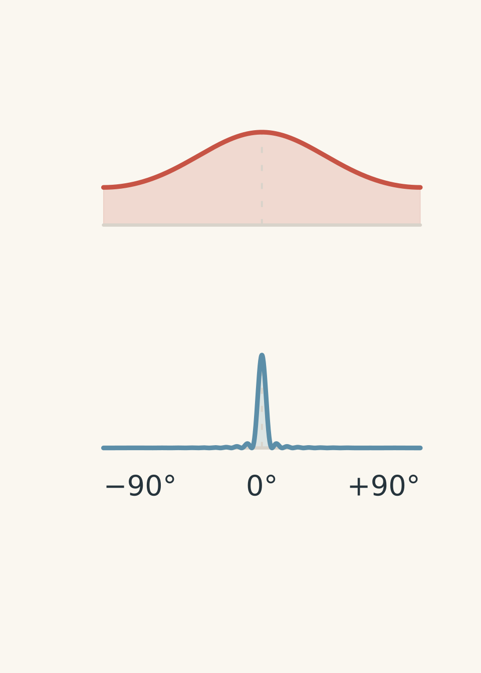
(c) Two openings have widths of \(0.5\lambda\) and \(10\lambda\), respectively. Compare the spreading of light through these openings and explain the difference. (2 marks)
(d) A diffraction grating has 500 lines per millimetre. A first-order maximum occurs at an angle of \(17.5^\circ\).
Calculate the wavelength of the incident light. (2 marks)
(e) A diffraction grating must just resolve two wavelengths, \(589.0\ \mathrm{nm}\) and \(589.6\ \mathrm{nm}\), in second order.
The resolving power is given by
\[ R=\frac{\lambda}{\Delta\lambda}=mN \]
where \(\lambda\) is the mean wavelength, \(\Delta\lambda\) is the wavelength separation, \(m\) is the order, and \(N\) is the number of illuminated lines.
Calculate the minimum whole number of illuminated lines required. Explain why increasing the number of illuminated lines improves wavelength resolution. (3 marks)
Question 3 (11 marks)
(a) Distinguish between continuous, emission-line, and absorption-line spectra. For each type, describe its physical origin. (3 marks)
(b) The intensity spectrum of a star peaks at a wavelength of \(480\ \mathrm{nm}\).
Using Wien’s displacement law,
\[ \lambda_{\max}T=b \]
calculate the star’s surface temperature. (2 marks)
(c) Spectral analysis of a star reveals absorption lines matching laboratory spectra of helium and sodium. Several pressure-sensitive lines are also broader than expected.
What can these observations tell an astronomer about the star’s atmospheric composition and density or pressure? (2 marks)
(d) A spectral line has a laboratory rest wavelength of \(500.0\ \mathrm{nm}\). In a distant galaxy, the line is observed at \(500.8\ \mathrm{nm}\).
Calculate the galaxy’s radial speed and state whether it is approaching or receding. Use
\[ \frac{v}{c}\approx\frac{\Delta\lambda}{\lambda_0} \]
where \(\lambda_0\) is the rest wavelength. (2 marks)
(e) A spectral line with a rest wavelength of \(600\ \mathrm{nm}\) is broadened symmetrically, with its edges shifted by \(+0.12\ \mathrm{nm}\) and \(-0.12\ \mathrm{nm}\) relative to the rest wavelength.
Estimate the star’s projected rotation speed and explain why rotation broadens spectral lines. (2 marks)
Question 4 (10 marks)
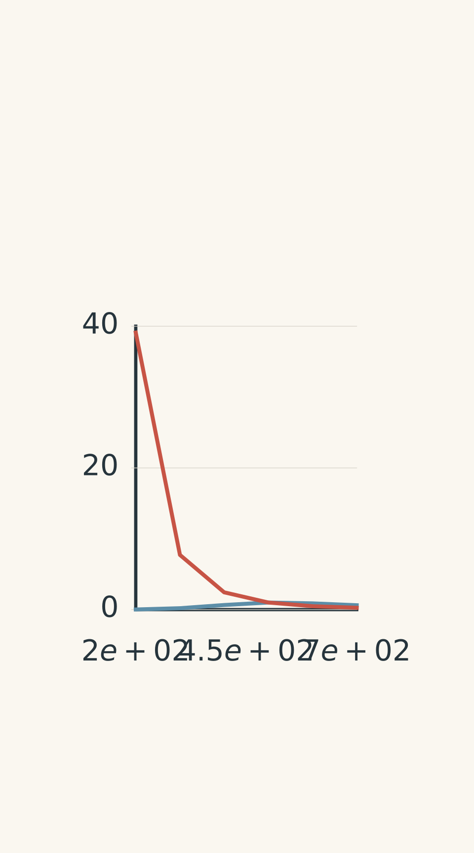
(a) The following illustrative data show two candidate predictions, A and B, for the spectral intensity of black-body radiation at different wavelengths. The intensities are in arbitrary relative units.
| Wavelength (nm) | Curve A | Curve B |
|---|---|---|
| 200 | 0.02 | 39.1 |
| 300 | 0.20 | 7.72 |
| 400 | 0.65 | 2.44 |
| 500 | 1.00 | 1.00 |
| 600 | 0.88 | 0.48 |
| 700 | 0.62 | 0.26 |
- A
- B
Identify the curve that matches observed black-body spectra. Explain what is wrong with the classical prediction and how Planck’s idea of quantised energy addressed the problem. (3 marks)
(b) Light of frequency \(8.0\times10^{14}\ \mathrm{Hz}\) shines on a metal with work function \(\phi=2.4\ \mathrm{eV}\).
Using the photoelectric equation
\[ K_{\max}=hf-\phi \]
calculate the maximum kinetic energy of the emitted electrons in joules and electronvolts. (3 marks)
(c) In a photoelectric experiment, no electrons are emitted when the incident frequency is below a particular threshold, even when the light intensity is increased. Above the threshold, emission occurs without a measurable delay.
Explain how these observations support the photon model of light and challenge the classical wave model. (2 marks)
(d) The frequency of light incident on a metal remains constant and is above the threshold frequency. The light intensity is doubled.
State what happens to the maximum kinetic energy of the emitted electrons and the rate of electron emission. Explain your answer. (2 marks)
Question 5 (10 marks)
(a) Two events occur at the same location inside a spacecraft. A clock at that location records a proper time interval of \(2.40\ \mathrm{\mu s}\) between them.
The spacecraft moves at \(0.80c\) relative to Earth.
Calculate the time interval measured by an observer on Earth. (3 marks)
(b) Cosmic muons have a proper mean lifetime of \(2.20\ \mathrm{\mu s}\) and travel at \(0.995c\) relative to Earth.
Calculate:
- the Lorentz factor;
- the mean lifetime measured in Earth’s frame;
- the average distance travelled before decay.
Explain how your result helps account for muons being detected at Earth’s surface. (4 marks)
(c) In a Hafele-Keating-style test, atomic clocks are flown eastward and westward around Earth and compared with a reference clock kept on the ground.
Explain what this comparison tests and why the relativistic prediction must account for both motion and gravitational potential. (2 marks)
(d) Define proper time. (1 mark)
Question 6 (10 marks)
(a) A rod has a rest length of \(2.40\ \mathrm{m}\). It moves at \(0.80c\) relative to a stationary observer, with its length parallel to its direction of motion.
Calculate the length measured by the stationary observer and identify the proper length. (2 marks)
(b) A proton of mass \(1.67\times10^{-27}\ \mathrm{kg}\) moves at \(0.90c\).
Using the relativistic momentum equation
\[ p=\gamma mv \]
calculate its momentum. (3 marks)
(c) In a particle accelerator, supplying more energy to a proton already moving close to \(c\) causes its energy and momentum to rise substantially, while its speed increases only slightly.
Explain why this supports relativity and state the limiting speed predicted by special relativity. (2 marks)
(d) An electron and a positron, each initially at rest, annihilate. Assume their entire rest-mass energy is converted into two photons emitted in opposite directions.
Calculate the total energy released and the energy of each photon. Give your answers in joules and, where appropriate, megaelectronvolts. (3 marks)
Question 7 (8 marks)
(a) Explain why the polarisation of light supports the model of light as a transverse wave rather than a longitudinal wave. (2 marks)
(b) Plane-polarised light with intensity \(I_{\max}=150\ \mathrm{W\,m^{-2}}\) reaches an analyser. The angle between the light’s polarisation direction and the analyser’s transmission axis is \(40^\circ\).
Using Malus’ law,
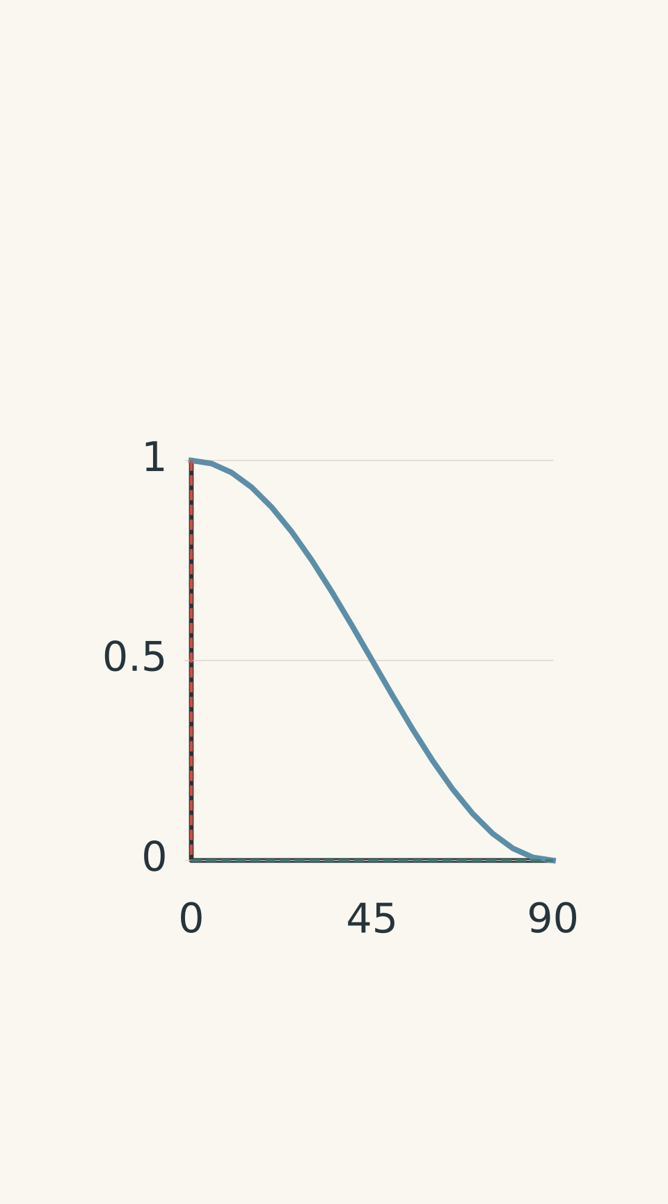
\[ I=I_{\max}\cos^2\theta \]
calculate the transmitted intensity. (3 marks)
(c) In a separate measurement, the same initial intensity, \(I_{\max}=150\ \mathrm{W\,m^{-2}}\), produces a transmitted intensity of \(38\ \mathrm{W\,m^{-2}}\).
Determine the angle between the polarisation direction and the analyser’s transmission axis, taking the angle to lie between \(0^\circ\) and \(90^\circ\). (3 marks)
Question 8 (8 marks)
(a) Describe how Fizeau’s rotating toothed-wheel method was used to measure the speed of light. State one limitation of the method. (2 marks)
(b) In a frequency-wavelength method, a laser has a vacuum frequency of \(5.00\times10^{14}\ \mathrm{Hz}\) and a vacuum wavelength of \(599.6\ \mathrm{nm}\).
Using \(c=f\lambda\), calculate the corresponding wave speed. (2 marks)
(c) Compared with Fizeau’s method, explain one reason later laser-frequency and wavelength techniques can provide more precise results. (2 marks)
(d) In the modern SI, the speed of light in vacuum is fixed at exactly \(299\,792\,458\ \mathrm{m\,s^{-1}}\).
Explain how this definition links length to time and why modern practice realises the metre using time and frequency standards rather than experimentally determining \(c\) as an unknown constant. (2 marks)
03Worked solutions and marking guide
Award marks for the specific steps and ideas listed below. Accept mathematically equivalent methods and reasonable rounding. Award follow-through marks where a student’s method remains valid when applied to their own earlier numerical result.
Solution 1
(a) Einstein’s postulates and evidence (3 marks)
The two postulates are:
- The laws of physics are the same in all inertial reference frames. No inertial frame is physically preferred.
- The speed of light in vacuum has the same value for all inertial observers, independent of the motion of the source or observer.
One relevant piece of evidence is the Michelson-Morley experiment. It failed to detect the expected variation in light speed associated with Earth’s motion through a hypothetical luminiferous ether. This result was consistent with the absence of a preferred ether frame and supported the invariant-light-speed postulate.
Marking:
- 1 mark for the first postulate.
- 1 mark for the second postulate.
- 1 mark for relevant experimental evidence and its connection to invariant light speed.
(b) Maxwell’s prediction of the speed of light (2 marks)
Substitute the given vacuum constants into the equation.
\[ c=\frac{1}{\sqrt{\mu_0\epsilon_0}} \]
\[ c=\frac{1}{ \sqrt{(4\pi\times10^{-7})(8.85\times10^{-12})} } \]
\[ c\approx2.998\times10^8\ \mathrm{m\,s^{-1}} \]
To three significant figures,
\[ \boxed{c=3.00\times10^8\ \mathrm{m\,s^{-1}}} \]
This prediction showed that electromagnetic theory naturally produces a wave speed equal to the measured speed of light.
Marking:
- 1 mark for correct substitution into the equation.
- 1 mark for the correct numerical value and unit.
(c) Maxwell’s electromagnetic theory (3 marks)
Maxwell unified electricity and magnetism by showing that electric and magnetic fields are linked. A changing magnetic field can induce an electric field, while a changing electric field contributes to the magnetic field.
Accelerating charges can produce electromagnetic disturbances. These disturbances propagate as electromagnetic waves, with the electric field and magnetic field perpendicular to each other and to the direction of travel. The waves carry energy through space.
Marking:
- 1 mark for explaining the linked, changing electric and magnetic fields.
- 1 mark for identifying accelerating charges as a source of electromagnetic waves.
- 1 mark for the transverse field arrangement and energy propagation.
(d) Huygens’ wave model (2 marks)
Huygens proposed that every point on a wavefront acts as a source of secondary wavelets. The envelope of these wavelets forms the next wavefront.
This construction accounts for diffraction: light spreads into regions beyond the direct path through a narrow opening. Interference patterns also support the wave model because overlapping waves can reinforce or cancel one another.
Marking:
- 1 mark for correctly describing the secondary-wavelet construction.
- 1 mark for connecting the model to diffraction or interference.
(e) Newton’s corpuscular model (2 marks)
Newton’s model treated light as particles travelling along paths. It described reflection successfully by treating light particles as bouncing from a surface.
However, diffraction and interference challenge a simple straight-line particle model. Light can spread beyond an opening and form alternating bright and dark fringes, behaviour explained naturally by a wave model.
Marking:
- 1 mark for a valid success, such as reflection.
- 1 mark for a valid limitation, such as diffraction or interference.
Solution 2
(a) Second-order double-slit maximum (2 marks)
Convert the quantities into metres.
\[ d=0.30\ \mathrm{mm}=3.00\times10^{-4}\ \mathrm{m} \]
\[ \lambda=600\ \mathrm{nm}=6.00\times10^{-7}\ \mathrm{m} \]
For the second-order maximum, \(m=2\).
\[ \sin\theta=\frac{m\lambda}{d} \]
\[ \sin\theta= \frac{2(6.00\times10^{-7})} {3.00\times10^{-4}} =0.00400 \]
Therefore,
\[ \theta=\sin^{-1}(0.00400) \]
\[ \boxed{\theta=0.229^\circ} \]
Marking:
- 1 mark for correct substitution, including unit conversions.
- 1 mark for the correct angle.
(b) Fringe position and spacing (2 marks)
The second-order maximum lies at angle \(\theta=0.229^\circ\). Its distance from the central maximum is
\[ y_2=L\tan\theta \]
\[ y_2=2.0\tan(0.229^\circ) \]
\[ y_2\approx0.00800\ \mathrm{m}=8.00\ \mathrm{mm} \]
The second-order maximum is two fringe spacings from the central maximum. Therefore,
\[ \Delta y=\frac{y_2}{2} \]
\[ \boxed{\Delta y=4.00\ \mathrm{mm}} \]
Marking:
- 1 mark for the correct second-order position.
- 1 mark for dividing by two to obtain the adjacent-fringe spacing.
(c) Diffraction through narrow openings (2 marks)
The opening of width \(0.5\lambda\) produces much greater angular spreading than the opening of width \(10\lambda\).
Diffraction becomes more pronounced when the opening width is comparable to or smaller than the wavelength. A much wider opening produces a narrower spread of light.
Marking:
- 1 mark for correctly comparing the two openings.
- 1 mark for explaining the relationship between opening width and diffraction.
(d) Diffraction-grating wavelength (2 marks)
The grating has 500 lines per millimetre. Its line spacing is
\[ d=\frac{1}{500}\ \mathrm{mm} =2.00\times10^{-6}\ \mathrm{m} \]
For a first-order maximum, \(m=1\).
\[ d\sin\theta=m\lambda \]
\[ \lambda=d\sin17.5^\circ \]
\[ \lambda=(2.00\times10^{-6})\sin17.5^\circ \]
\[ \boxed{\lambda=6.02\times10^{-7}\ \mathrm{m} =602\ \mathrm{nm}} \]
Marking:
- 1 mark for finding the grating spacing.
- 1 mark for the correct wavelength and unit.
(e) Grating resolving power (3 marks)
The mean wavelength is
\[ \lambda=\frac{589.0+589.6}{2} =589.3\ \mathrm{nm} \]
The wavelength separation is
\[ \Delta\lambda=589.6-589.0 =0.6\ \mathrm{nm} \]
Therefore,
\[ R=\frac{\lambda}{\Delta\lambda} =\frac{589.3}{0.6} \approx982 \]
Since \(R=mN\), and the order is \(m=2\),
\[ N=\frac{R}{m} =\frac{982.17}{2} \approx491.1 \]
The number of lines must be a whole number, so the minimum is
\[ \boxed{N=492\text{ illuminated lines}} \]
More illuminated lines produce narrower principal maxima. The smaller the width of these maxima, the easier it is to distinguish two nearby wavelengths.
Marking:
- 1 mark for calculating the resolving power.
- 1 mark for finding \(N\) and rounding up to 492.
- 1 mark for explaining why more illuminated lines improve resolution.
Solution 3
(a) Types of spectra (3 marks)
- A continuous spectrum contains a broad, uninterrupted range of wavelengths. It is produced by a hot, dense source, such as a hot solid or dense gas.
- An emission-line spectrum contains bright lines at particular wavelengths. It is produced when excited atoms or ions in a relatively low-density gas emit photons at specific energies.
- An absorption-line spectrum contains dark lines within a continuous spectrum. It forms when cooler gas absorbs particular wavelengths from light passing through it.
Marking:
- 1 mark for each spectrum type and its physical origin.

(b) Stellar surface temperature (2 marks)
Wien’s displacement law is
\[ \lambda_{\max}T=b \]
Rearranging,
\[ T=\frac{b}{\lambda_{\max}} \]
Substitute \(\lambda_{\max}=480\ \mathrm{nm} =4.80\times10^{-7}\ \mathrm{m}\).
\[ T=\frac{2.90\times10^{-3}} {4.80\times10^{-7}} \]
\[ \boxed{T=6.04\times10^3\ \mathrm{K}} \]
The star’s estimated surface temperature is approximately \(6040\ \mathrm{K}\).
Marking:
- 1 mark for the correct equation and unit conversion.
- 1 mark for the correct temperature.
(c) Composition and atmospheric density (2 marks)
The matching absorption lines indicate that helium and sodium are present in the star’s atmosphere. Each element has a characteristic pattern of spectral lines, which acts as a chemical fingerprint.
The unusually broad pressure-sensitive lines suggest relatively high atmospheric pressure or density. Collisions between particles can broaden spectral lines, although other broadening mechanisms must also be considered when analysing a real star.
Marking:
- 1 mark for identifying composition from characteristic line wavelengths.
- 1 mark for linking pressure-sensitive line broadening to atmospheric pressure or density.
(d) Radial velocity (2 marks)
The wavelength shift is
\[ \Delta\lambda=500.8-500.0=0.8\ \mathrm{nm} \]
Using the supplied approximation,
\[ v=c\frac{\Delta\lambda}{\lambda_0} \]
\[ v=3.00\times10^8 \left(\frac{0.8}{500.0}\right) \]
\[ \boxed{v=4.80\times10^5\ \mathrm{m\,s^{-1}}} \]
This is \(480\ \mathrm{km\,s^{-1}}\).
The observed wavelength is longer than the rest wavelength, so the line is redshifted. The galaxy is receding.
Marking:
- 1 mark for the correct radial speed.
- 1 mark for identifying the direction from the redshift.
(e) Rotational broadening (2 marks)
Use the shift at either edge of the line:
\[ \Delta\lambda=0.12\ \mathrm{nm}, \qquad \lambda_0=600\ \mathrm{nm} \]
\[ v\approx c\frac{\Delta\lambda}{\lambda_0} \]
\[ v=3.00\times10^8 \left(\frac{0.12}{600}\right) \]
\[ \boxed{v=6.00\times10^4\ \mathrm{m\,s^{-1}} =60.0\ \mathrm{km\,s^{-1}}} \]
One side of a rotating star moves towards the observer, producing a blueshift. The opposite side moves away, producing a redshift. Light from both sides contributes to the observed spectrum, broadening the line.
Marking:
- 1 mark for the correct projected rotation speed.
- 1 mark for explaining the opposing Doppler shifts across the rotating star.
Solution 4
(a) Black-body radiation and Planck’s quantisation (3 marks)
Curve A matches observed black-body spectra. Its intensity rises to a peak and then falls at shorter wavelengths. Real black bodies do not emit an unlimited amount of energy at increasingly short wavelengths.
Curve B represents the classical prediction associated with the ultraviolet catastrophe. Classical theory predicted that the spectral intensity would grow without bound towards very short wavelengths, contradicting observation.
Planck resolved the problem by proposing that energy exchange occurs in discrete quanta. For an oscillator of frequency \(f\), the allowed energy levels are separated by
\[ E=hf \]
High-frequency oscillations require larger energy quanta. This quantisation leads to the observed fall-off at short wavelengths rather than the classical divergence.
Marking:
- 1 mark for identifying Curve A as the observed spectrum and describing its peak and fall-off.
- 1 mark for explaining the classical ultraviolet catastrophe.
- 1 mark for explaining how quantised energy addressed the discrepancy.
(b) Maximum photoelectron kinetic energy (3 marks)
The photoelectric equation is
\[ K_{\max}=hf-\phi \]
First calculate the energy of one photon:
\[ hf=(6.63\times10^{-34})(8.0\times10^{14}) \]
\[ hf=5.304\times10^{-19}\ \mathrm{J} \]
Convert the work function into joules:
\[ \phi=2.4(1.60\times10^{-19}) \]
\[ \phi=3.84\times10^{-19}\ \mathrm{J} \]
Therefore,
\[ \begin{aligned} K_{\max} &=5.304\times10^{-19} -3.84\times10^{-19}\\ &=1.464\times10^{-19}\ \mathrm{J} \end{aligned} \]
Convert to electronvolts:
\[ K_{\max} =\frac{1.464\times10^{-19}} {1.60\times10^{-19}} \]
\[ \boxed{K_{\max}=1.46\times10^{-19}\ \mathrm{J} =0.915\ \mathrm{eV}} \]
Marking:
- 1 mark for applying the photoelectric equation.
- 1 mark for correctly calculating the photon energy and converting the work function.
- 1 mark for the correct kinetic energy, with units.
(c) Threshold frequency and immediate emission (2 marks)
In the photon model, each photon carries energy \(E=hf\). An electron can escape only if the photon supplies at least the work function of the metal.
Below the threshold frequency, increasing intensity adds more photons but does not increase the energy of each photon. Above threshold, a single photon can transfer enough energy to release an electron, explaining why emission occurs without a measurable accumulation delay.
Marking:
- 1 mark for explaining the threshold using photon energy and work function.
- 1 mark for explaining the immediate emission and contrast with the classical wave prediction.
(d) Increasing light intensity (2 marks)
The maximum kinetic energy remains unchanged because the frequency is unchanged:
\[ K_{\max}=hf-\phi \]
The rate of electron emission increases because greater intensity at the same frequency means more photons arriving per second. More photons can release more electrons, but each photon still has the same energy.
Marking:
- 1 mark for stating that the maximum kinetic energy is unchanged.
- 1 mark for explaining that the emission rate increases because the photon flux increases.
Solution 5
(a) Time dilation (3 marks)
The proper time is
\[ \Delta\tau=2.40\ \mathrm{\mu s} \]
The Lorentz factor is
\[ \gamma=\frac{1}{\sqrt{1-v^2/c^2}} \]
At \(v=0.80c\),
\[ \gamma=\frac{1}{\sqrt{1-0.80^2}} =\frac{1}{0.60} =1.667 \]
The time interval measured on Earth is
\[ \Delta t=\gamma\Delta\tau \]
\[ \Delta t=1.667(2.40\ \mathrm{\mu s}) \]
\[ \boxed{\Delta t=4.00\ \mathrm{\mu s}} \]
The Earth observer measures a longer interval than the clock moving with the spacecraft.
Marking:
- 1 mark for calculating the Lorentz factor.
- 1 mark for applying the time-dilation relationship.
- 1 mark for the correct time interval.
(b) Cosmic muons (4 marks)
The muon’s proper mean lifetime is
\[ \tau_0=2.20\ \mathrm{\mu s} \]
At \(v=0.995c\), the Lorentz factor is
\[ \gamma=\frac{1}{\sqrt{1-0.995^2}} \]
\[ \gamma=\frac{1}{\sqrt{0.009975}} \approx10.0 \]
The mean lifetime measured in Earth’s frame is
\[ \tau=\gamma\tau_0 \]
\[ \tau\approx10.0125(2.20\ \mathrm{\mu s}) \]
\[ \tau\approx22.0\ \mathrm{\mu s} \]
The average distance travelled is
\[ d=v\tau \]
\[ d=(0.995)(3.00\times10^8) (22.0275\times10^{-6}) \]
\[ \boxed{d\approx6.58\times10^3\ \mathrm{m} =6.58\ \mathrm{km}} \]
Without time dilation, the distance corresponding to the proper mean lifetime would be only about \(657\ \mathrm{m}\). Time dilation therefore explains how many fast-moving muons can travel several kilometres through the atmosphere before decaying, allowing some to reach ground-level detectors.
Marking:
- 1 mark for the correct Lorentz factor.
- 1 mark for the dilated mean lifetime.
- 1 mark for the average travel distance with units.
- 1 mark for connecting time dilation to muon detection at Earth’s surface.
(c) Atomic-clock tests (2 marks)
The flown clocks are compared with a reference clock to test whether the observed time differences agree with relativistic predictions.
The predictions must include special-relativistic effects due to the clocks’ motion and general-relativistic effects due to differences in gravitational potential. The eastward and westward flights have different motions relative to Earth’s rotation, so their predicted clock shifts need not be the same. Agreement between measured and predicted differences supports relativity.
Marking:
- 1 mark for explaining the comparison and its purpose.
- 1 mark for identifying both motion-related and gravitational contributions.
(d) Proper time (1 mark)
Proper time is the time interval between two events measured in a reference frame in which both events occur at the same location.
Marking:
- 1 mark for the correct definition.
Solution 6
(a) Length contraction (2 marks)
The rod’s rest length is its proper length:
\[ L_0=2.40\ \mathrm{m} \]
The Lorentz factor at \(0.80c\) is
\[ \gamma=\frac{1}{\sqrt{1-0.80^2}}=1.667 \]
Length contraction gives
\[ L=\frac{L_0}{\gamma} \]
\[ L=\frac{2.40}{1.667} \]
\[ \boxed{L=1.44\ \mathrm{m}} \]
The proper length is \(2.40\ \mathrm{m}\), measured in the rod’s rest frame. The stationary observer measures the shorter length along the direction of motion.
Marking:
- 1 mark for applying length contraction correctly.
- 1 mark for the contracted length and correct identification of the proper length.
(b) Relativistic momentum (3 marks)
The proton’s speed is
\[ v=0.90c=2.70\times10^8\ \mathrm{m\,s^{-1}} \]
The Lorentz factor is
\[ \gamma=\frac{1}{\sqrt{1-0.90^2}} =\frac{1}{\sqrt{0.19}} \approx2.294 \]
Substitute into the relativistic momentum equation:
\[ p=\gamma mv \]
\[ p=(2.294)(1.67\times10^{-27}) (2.70\times10^8) \]
\[ \boxed{p=1.03\times10^{-18}\ \mathrm{kg\,m\,s^{-1}}} \]
Marking:
- 1 mark for calculating the Lorentz factor.
- 1 mark for correct substitution into the momentum equation.
- 1 mark for the correct momentum and unit.
(c) Particle accelerators and the speed limit (2 marks)
As a particle approaches the speed of light, its Lorentz factor increases rapidly. Additional energy produces substantial increases in relativistic energy and momentum, but progressively smaller increases in speed.
Reaching \(c\) would require unbounded energy for a particle with non-zero rest mass. Special relativity therefore predicts that such a particle cannot reach or exceed the speed of light in vacuum.
Marking:
- 1 mark for explaining the increase in energy and momentum at high speed.
- 1 mark for identifying \(c\) as the limiting speed and explaining why it cannot be reached by a massive particle.
(d) Electron-positron annihilation (3 marks)
Both particles have rest mass \(m_e\). The total initial rest-mass energy is
\[ E_{\mathrm{total}}=2m_ec^2 \]
Substituting the supplied values,
\[ E_{\mathrm{total}} =2(9.11\times10^{-31})(3.00\times10^8)^2 \]
\[ \boxed{E_{\mathrm{total}}=1.64\times10^{-13}\ \mathrm{J}} \]
This corresponds to approximately \(1.02\ \mathrm{MeV}\).
The two photons share the energy equally because the initial system is at rest and the photons are emitted in opposite directions. Each photon has energy
\[ E_\gamma=\frac{E_{\mathrm{total}}}{2} \]
\[ \boxed{E_\gamma=8.20\times10^{-14}\ \mathrm{J} \approx0.512\ \mathrm{MeV}} \]
The opposite photon momenta conserve the initial total momentum of zero.
Marking:
- 1 mark for applying \(E=mc^2\) to both particles.
- 1 mark for the correct total energy.
- 1 mark for the energy per photon, with appropriate units.
Solution 7
(a) Polarisation and transverse waves (2 marks)
Polarisation restricts the direction in which the electric field of light oscillates. These oscillations are perpendicular to the direction in which the light travels.
A longitudinal wave oscillates parallel to its direction of travel and cannot be polarised in this way. The existence of polarisation therefore supports the conclusion that light is a transverse wave.
Marking:
- 1 mark for describing polarisation as a restriction of the oscillation direction.
- 1 mark for connecting this behaviour to the transverse nature of light.
(b) Malus’ law (3 marks)
Malus’ law gives the transmitted intensity:
\[ I=I_{\max}\cos^2\theta \]
Substitute the given values:
\[ I=150\cos^2 40^\circ \]
Since \(\cos40^\circ\approx0.766\),
\[ I=150(0.766)^2 \]
\[ \boxed{I=88.0\ \mathrm{W\,m^{-2}}} \]
The analyser transmits less intensity because its transmission axis is not aligned with the incoming polarisation direction.
Marking:
- 1 mark for selecting the correct relationship.
- 1 mark for correct substitution.
- 1 mark for the numerical result and unit.
(c) Finding the angle from intensity (3 marks)
Start with Malus’ law:
\[ I=I_{\max}\cos^2\theta \]
Rearrange:
\[ \cos^2\theta=\frac{I}{I_{\max}} \]
\[ \cos^2\theta=\frac{38}{150}=0.2533 \]
Taking the square root,
\[ \cos\theta=\sqrt{0.2533}\approx0.5033 \]
Therefore,
\[ \theta=\cos^{-1}(0.5033) \]
\[ \boxed{\theta=59.8^\circ} \]
Marking:
- 1 mark for correctly rearranging Malus’ law.
- 1 mark for correctly taking the square root and applying the inverse cosine.
- 1 mark for the correct angle.
- I/I_max = cos²θ
- Maximum
- Zero transmission
Solution 8
(a) Fizeau’s toothed-wheel method (2 marks)
Fizeau directed light through a gap in a rotating toothed wheel towards a distant mirror. The light reflected back towards the wheel could be blocked by a tooth if the wheel rotated sufficiently during the light’s round trip.
The wheel’s rotation rate and the distance to the mirror allowed the round-trip travel time to be calculated. Dividing the total distance travelled by this time gave an estimate of the speed of light.
One limitation was the difficulty of measuring the rotation rate and detecting the precise extinction condition. Alignment and uncertainty in the long optical path also affected accuracy.
Marking:
- 1 mark for describing the wheel, mirror, and returning light.
- 1 mark for explaining how the travel time was inferred or identifying a valid limitation.
(b) Frequency-wavelength calculation (2 marks)
Convert the wavelength into metres:
\[ \lambda=599.6\ \mathrm{nm} =5.996\times10^{-7}\ \mathrm{m} \]
Use the wave relationship:
\[ c=f\lambda \]
\[ c=(5.00\times10^{14}) (5.996\times10^{-7}) \]
\[ \boxed{c=2.998\times10^8\ \mathrm{m\,s^{-1}}} \]
This is consistent with the accepted speed of light in vacuum.
Marking:
- 1 mark for converting the wavelength and applying the correct equation.
- 1 mark for the correct result and unit.
(c) Comparing measurement methods (2 marks)
Fizeau’s method depended on a mechanical rotation rate and the time taken for light to travel along a long path and return. Uncertainty in these measurements limited its precision.
Later laser-frequency and wavelength techniques could use stable frequency references and precise optical interference measurements. Counting or measuring many optical cycles allowed much smaller uncertainties than relying on mechanical rotation and a long-path extinction measurement.
Marking:
- 1 mark for a valid comparison of the quantities measured.
- 1 mark for explaining a specific precision advantage of later optical techniques.
(d) The speed of light and the modern SI (2 marks)
The second is defined using a specified frequency of radiation associated with caesium-133. The metre is defined as the distance light travels in vacuum during \(1/299\,792\,458\) of a second.
Fixing \(c\) at exactly \(299\,792\,458\ \mathrm{m\,s^{-1}}\) links the realisation of length to the unit of time. Modern laboratories use time and frequency standards, together with suitable optical measurement techniques, to realise the metre. They do not experimentally determine \(c\) as an unknown constant in the modern SI.
Marking:
- 1 mark for explaining how the metre is linked to the second through the fixed value of \(c\).
- 1 mark for explaining why modern practice realises the metre rather than remeasuring \(c\) as an unknown constant.