
Three Ways Magnetic Flux Can Change Without Moving a Magnet
Learn how magnetic flux changes when field strength, loop area, or orientation changes, even when the magnet stays still. Work through HSC Physics examples, avoid the plane-versus-normal angle trap, and practise applying Faraday’s law.
In an HSC Physics response, you might write, “There is no induced emf because the magnet isn’t moving.” It sounds reasonable, but it confuses one way of changing magnetic flux with the actual condition for electromagnetic induction.
A magnet can stay completely still while the magnetic flux through a coil changes.
Predict what happens in these three situations. The field source stays in place, but you increase the current through an electromagnet, squeeze a wire loop into a smaller shape, or tilt a coil in a magnetic field. Can any of these produce an induced emf?
Yes. All three can, provided they change the magnetic flux through the coil. The trick is to stop asking whether the magnet moves and start checking what happens to the flux.
Three ways to change magnetic flux
| A — Field strength B | Φ_B = BA cos θ Increase B; keep the coil stationary. A and θ stay constant, so flux increases. |
|---|---|
| B — Enclosed area A | Φ_B = BA cos θ Slide one side of the rectangular loop inward. B and θ stay constant; decreasing A decreases flux magnitude when cos θ ≠ 0. |
| C — Orientation θ | Φ_B = BA cos θ Tilt the coil in an unchanged magnetic field. B and A stay constant; changing θ changes flux unless the relevant cosine values are equal. |
01The rule that catches the mistake
Imagine holding a window in the rain. More intense rain means more water passes through it. A larger window catches more water, and tilting the window changes how much rain passes through its opening.
Magnetic flux works in a similar way. You can change it by changing the field strength, the area enclosed by the loop, or the loop’s orientation relative to the field.
The analogy has limits: magnetic field lines are not literal threads passing through the loop, and magnetic flux can be positive or negative depending on the chosen direction of the loop’s normal.
For a flat loop in a uniform magnetic field, magnetic flux is calculated using
\[ \Phi_B=BA\cos\theta \]
where:
- \(\Phi_B\) is the magnetic flux through one turn, measured in webers (Wb).
- \(B\) is the magnetic field strength, measured in teslas (T).
- \(A\) is the area enclosed by the loop, measured in square metres (\(\mathrm{m^2}\)).
- \(\theta\) is the angle between the magnetic field and the loop’s area normal.
The area normal is an imaginary line perpendicular to the plane of the loop. It is not a line that lies along the wire.
For a coil with \(N\) turns, Faraday’s law gives the average induced emf:
\[ \mathcal E_{\mathrm{avg}} =-N\frac{\Delta\Phi_B}{\Delta t} \]
Here, \(N\) is the number of turns, \(\Delta\Phi_B=\Phi_f-\Phi_i\) is the change in flux per turn, and \(\Delta t\) is the time interval in seconds. The induced emf, \(\mathcal E_{\mathrm{avg}}\), is measured in volts (V).
The minus sign represents Lenz’s law: the induced current, when there is a closed conducting path, produces a magnetic field that opposes the change in magnetic flux.
For the magnitude of the average emf, use
\[ |\mathcal E_{\mathrm{avg}}| =N\frac{|\Delta\Phi_B|}{\Delta t} \]
Keep this distinction in mind throughout the article: flux is what passes through the loop; induced emf depends on how that flux changes.
02Three ways to change magnetic flux
1. Change the field strength while the coil stays fixed
Imagine a coil beside a stationary electromagnet. The coil does not move, its enclosed area stays constant, and its orientation does not change.
Now increase the current through the electromagnet. Its magnetic field becomes stronger, so the magnetic flux through the coil changes.
Increasing magnetic field strength changes flux
| Initial instant | Φ_i = B_i A cos θ The electromagnet and coil are stationary. The initial magnetic field strength is B_i. |
|---|---|
| Later instant | Φ_f = B_f A cos θ B_f > B_i; the field through the unchanged coil is stronger. A and θ remain constant, so the flux increases. |
Because the area and angle remain constant, the flux is directly proportional to the field strength:
\[ \Phi_B=BA\cos\theta \]
If \(A\) and \(\theta\) stay fixed while \(B\) increases, \(\Phi_B\) increases too.
Notice what caused the induction. The current through the electromagnet changed, which changed the field strength. The magnet itself did not need to move.
A stationary permanent magnet with a stationary coil and no other changing conditions would not produce a sustained induced emf. A stationary field source, however, does not guarantee a stationary field.
Worked example: a changing field with a stationary coil
A 120-turn coil has an area of \(1.5\times10^{-2}\,\mathrm{m^2}\). Its normal is parallel to a uniform magnetic field produced by a stationary electromagnet. The field strength falls from \(0.50\,\mathrm T\) to \(0.20\,\mathrm T\) in \(0.10\,\mathrm s\). Calculate the magnitude of the average induced emf.
Step 1
The field is parallel to the normal, so \(\theta=0^\circ\) and \(\cos0^\circ=1\).
\[ \begin{aligned} \Phi_i&=(0.50)(0.015)\cos0^\circ\\ &=0.0075\ \mathrm{Wb} \end{aligned} \]
\[ \begin{aligned} \Phi_f&=(0.20)(0.015)\cos0^\circ\\ &=0.0030\ \mathrm{Wb} \end{aligned} \]
Step 2
\[ \begin{aligned} \Delta\Phi_B&=\Phi_f-\Phi_i\\ &=0.0030-0.0075\\ &=-0.0045\ \mathrm{Wb} \end{aligned} \]
The negative sign tells us that the flux has decreased.
Step 3
\[ \begin{aligned} |\mathcal E_{\mathrm{avg}}| &=N\frac{|\Delta\Phi_B|}{\Delta t}\\ &=\frac{120(0.0045)}{0.10}\\ &=5.4\ \mathrm V \end{aligned} \]
The average induced emf is \(5.4\,\mathrm V\).
The important result is not just the number. The coil and electromagnet remained in place, yet changing the field strength produced an emf. Once the field stops changing, the induced emf ceases, even though the coil still has magnetic flux through it.
2. Change the area enclosed by the loop
Now keep the magnetic field and the loop’s orientation fixed, but change the shape of the wire loop.
For example, imagine a rectangular loop with one side that can slide. Moving that side changes the area enclosed by the wire.
Reducing loop area changes magnetic flux
| Initial position | Φ₁ = BA₁ cos θ The sliding side is farther from the fixed side. The enclosed area is larger: A₁. |
|---|---|
| Final position | Φ₂ = BA₂ cos θ The sliding side moves inward; A₂ < A₁. With B and θ unchanged, the flux magnitude decreases if cos θ ≠ 0. |
The magnetic field has not changed, and the angle between the field and the normal is still the same. However, the enclosed area has changed.
With \(B\) and \(\theta\) constant,
\[ \Phi_B=BA\cos\theta \]
shows that flux is directly proportional to \(A\).
If the enclosed area decreases, the flux magnitude decreases, provided the field has a non-zero component perpendicular to the loop.
A common mistake is to look at the amount of wire and assume that the flux must stay constant if the wire’s total length stays constant. That is incorrect. Magnetic flux depends on the area enclosed by the loop, not its perimeter.
This is why reshaping a square loop into a rectangle can induce an emf even when the total length of wire remains unchanged.
3. Change the angle between the field and the area normal
The third option is to rotate the coil in a fixed magnetic field.
The coil’s actual area can remain exactly the same. What changes is its orientation relative to the field.
Coil orientation changes magnetic flux
| View 1 — Normal parallel to B | θ = 0°; Φ₁ = BA B is perpendicular to the coil’s plane. Magnetic flux magnitude is maximum. |
|---|---|
| View 2 — Normal at 60° to B | θ = 60°; Φ₂ = 0.5BA The normal remains perpendicular to the tilted coil’s plane. B makes 30° with the plane; flux magnitude is half the initial value. |
Return to the flux equation:
\[ \Phi_B=BA\cos\theta \]
If \(B\) and \(A\) stay constant, changing \(\theta\) changes the flux.
Two orientations are particularly useful to remember:
- When \(\theta=0^\circ\), the field is parallel to the normal and perpendicular to the plane of the loop. The flux magnitude is maximum: \(\Phi_B=BA\).
- When \(\theta=90^\circ\), the field is perpendicular to the normal and parallel to the plane of the loop. The flux is zero: \(\Phi_B=0\).
So, rotating a coil from the first orientation towards the second decreases the flux magnitude.
The coil moves during this process, but the magnet does not need to move. Once the coil stops rotating and its orientation becomes fixed, the induced emf ceases if the field and all other relevant conditions remain constant.
03The plane-versus-normal trap
This is one of the easiest ways to lose marks in a flux calculation.
The equation uses the angle between the magnetic field and the normal, not the angle between the magnetic field and the plane of the coil.
Measure the angle from the area normal
| 1. Field perpendicular to plane | θ = 0°; Φ_B = BA B is parallel to the area normal. Flux magnitude is maximum. |
|---|---|
| 2. Field parallel to plane | θ = 90°; Φ_B = 0 B is perpendicular to the area normal. Flux through the loop is zero. |
| 3. Field 30° to plane | θ = 60°; |Φ_B| = 0.5BA The normal is perpendicular to the coil’s plane. Measure θ between B and the normal, not the plane. |
Use this table to check your angle before substituting.
| Wording in the question | Angle \(\theta\) to use in \(\cos\theta\) | Flux magnitude |
|---|---|---|
| Field perpendicular to the plane | \(0^\circ\) | \(BA\) |
| Field parallel to the plane | \(90^\circ\) | \(0\) |
| Field \(30^\circ\) to the normal | \(30^\circ\) | \(BA\cos30^\circ\) |
| Field \(30^\circ\) to the plane | \(60^\circ\) | \(BA\cos60^\circ\) |
If a question gives the acute angle \(\alpha\) between the field and the plane, convert it before using the cosine formula:
\[ \theta=90^\circ-\alpha \]
Equivalently, the flux magnitude can be written as
\[ |\Phi_B|=BA\sin\alpha \]
when \(\alpha\) is the acute angle between the field and the plane.
Do not memorise the sine version as a separate rule without understanding where it comes from. The safest method is to draw the normal, mark the angle to the field, and use the formula you know.
Worked example: the area shrinks, but the flux increases
A 40-turn coil is in a uniform magnetic field of \(0.50\,\mathrm T\). Its area decreases from \(0.030\,\mathrm{m^2}\) to \(0.020\,\mathrm{m^2}\), while the field’s angle to the plane of the coil increases from \(30^\circ\) to \(60^\circ\). These changes occur over \(0.25\,\mathrm s\). Calculate the magnitude of the average induced emf.
Step 1
Initially,
\[ \theta_i=90^\circ-30^\circ=60^\circ \]
Finally,
\[ \theta_f=90^\circ-60^\circ=30^\circ \]
Step 2
\[ \begin{aligned} \Phi_i&=(0.50)(0.030)\cos60^\circ\\ &=7.50\times10^{-3}\ \mathrm{Wb} \end{aligned} \]
\[ \begin{aligned} \Phi_f&=(0.50)(0.020)\cos30^\circ\\ &=8.66\times10^{-3}\ \mathrm{Wb} \end{aligned} \]
Step 3
\[ \begin{aligned} \Delta\Phi_B &=(8.66-7.50)\times10^{-3}\\ &=1.16\times10^{-3}\ \mathrm{Wb} \end{aligned} \]
The flux has increased, even though the area has decreased.
Step 4
\[ \begin{aligned} |\mathcal E_{\mathrm{avg}}| &=\frac{40(1.16\times10^{-3})}{0.25}\\ &=0.186\ \mathrm V \end{aligned} \]
The average induced emf has a magnitude of \(0.186\,\mathrm V\).
Here is the tempting wrong approach: because the area decreases, you predict that the flux decreases. That ignores the angle change. The field becomes more perpendicular to the plane, increasing its component along the normal. In this example, that increase is large enough to outweigh the reduction in area.
There is a second trap. If you put \(30^\circ\) and \(60^\circ\) directly into \(\cos\theta\), you treat the angles to the plane as angles to the normal. You would predict the wrong change in flux and even the wrong polarity of the induced emf.
The corrected method is simple: convert the angles, calculate the initial and final flux separately, and only then subtract.
Changing area and orientation can increase magnetic flux
| Initial state | Φ_i = BA cos θ = 7.50 mWb A_i = 0.030 m²; B = 0.50 T. B is 30° to the plane, so θ = 60° to the normal. |
|---|---|
| Final state | Φ_f = BA cos θ = 8.66 mWb A_f = 0.020 m²; B remains 0.50 T. B is 60° to the plane, so θ = 30° to the normal. |
04Why non-zero magnetic flux does not mean there is an induced emf
Suppose a coil has a magnetic flux of \(0.002\,\mathrm{Wb}\) per turn. The field is non-zero, and magnetic flux passes through the coil.
If the field strength, area, and orientation remain constant, however, the flux stays at \(0.002\,\mathrm{Wb}\). No induced emf is produced.
Faraday’s law depends on the change in flux:
\[ \mathcal E_{\mathrm{avg}} =-N\frac{\Delta\Phi_B}{\Delta t} \]
If \(\Delta\Phi_B=0\), then
\[ \mathcal E_{\mathrm{avg}}=0 \]
The flux can be large, small, or non-zero without producing an induced emf. What matters is whether it changes.
This also explains why an emf does not continue simply because a coil has been left in a magnetic field. If the coil is rotated, an emf can be induced during the rotation. If it is then held still in the new orientation, the emf stops, even though the coil may still have substantial magnetic flux.
There is a subtle point worth remembering: zero flux at one instant does not necessarily mean zero induced emf at that instant. A rotating coil can pass through an orientation where its flux is zero while the flux is changing rapidly.
A more difficult case: several changes can cancel
You might now think that changing any one of \(B\), \(A\), or \(\theta\) must produce an emf. Not necessarily.
The three quantities combine in the same equation:
\[ \Phi_B=BA\cos\theta \]
If they change in a way that keeps \(BA\cos\theta\) constant, the magnetic flux does not change. There is no net induced emf around the loop, even though individual quantities are changing.
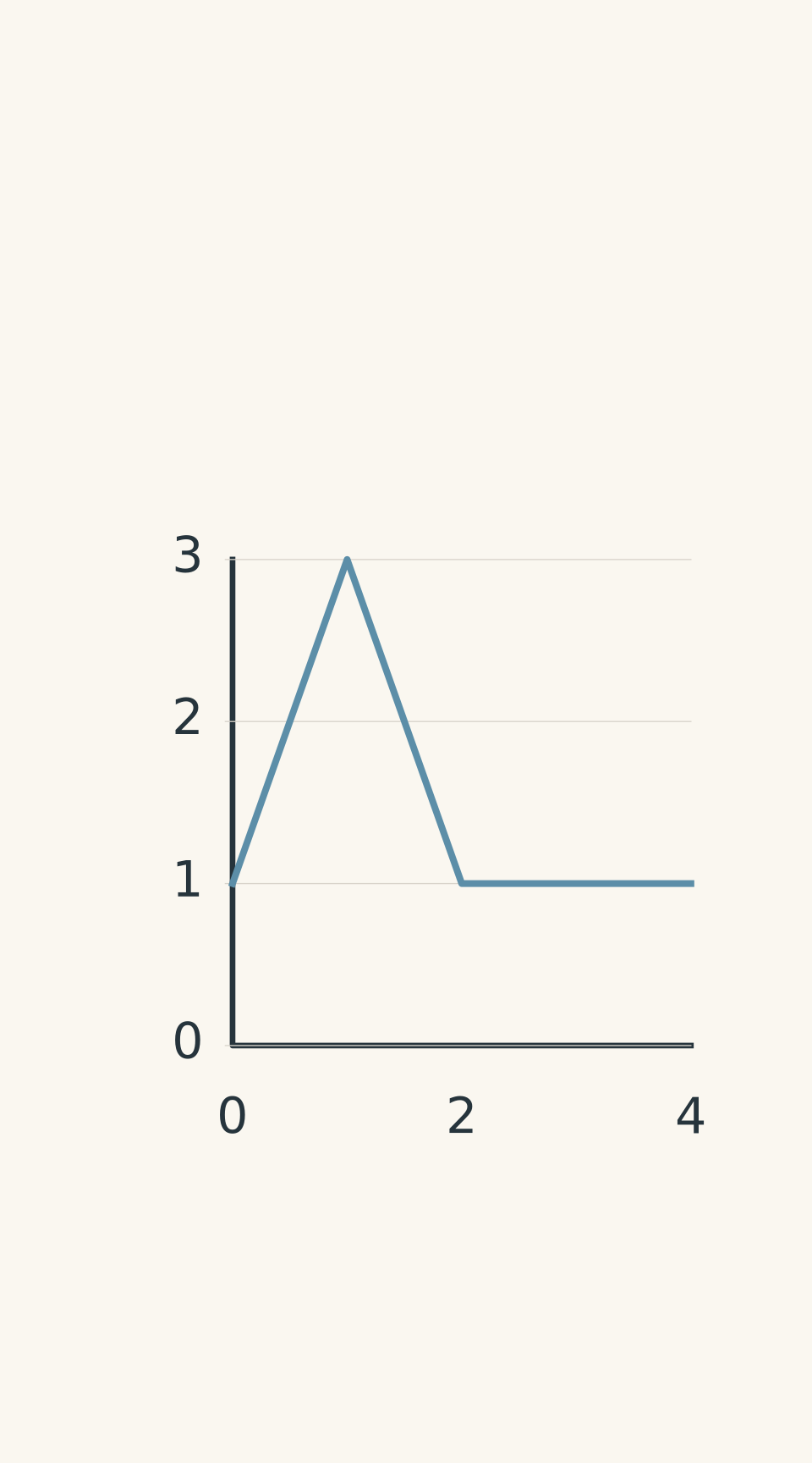
For example, if the field strength doubles while the angle changes from \(0^\circ\) to \(60^\circ\), the normal component of the field can remain constant:
\[ B_i\cos0^\circ=B_i \]
\[ B_f\cos60^\circ=(2B_i)(0.5)=B_i \]
With constant loop area, the flux is the same at both ends. If the relationship is maintained throughout the adjustment, the flux remains constant throughout, so the induced emf is zero.
- Flux per turn
Be careful with the phrase “the initial and final flux are equal”. That fact alone tells you the average emf over the entire interval is zero. It does not prove that the flux stayed constant between those endpoints. The flux could have increased and then decreased, producing non-zero emfs during both changes.
That distinction becomes important in harder exam questions.
05A decision method you can reuse in an exam
When you see a question about induced emf, work through this sequence.
- Draw the loop and its normal. Mark the magnetic field and identify the angle between the field and the normal.
- Identify what changes. Check the field strength, enclosed area, and orientation. Do not assume that the magnet must move.
- Calculate the initial flux. Use \(\Phi_i=B_iA_i\cos\theta_i\).
- Calculate the final flux. Use \(\Phi_f=B_fA_f\cos\theta_f\). If multiple quantities change, include all of them.
- Find the change in flux. Calculate \(\Delta\Phi_B=\Phi_f-\Phi_i\), then apply Faraday’s law using the number of turns and the time interval.
- Check the interpretation. A non-zero flux does not guarantee an emf. A changing field, area, or angle does not guarantee a net emf either if the changes cancel. If the question asks for direction, use Lenz’s law to determine how the induced field opposes the change in flux.
The key habit is to calculate flux at the relevant times rather than guessing from a single changing quantity.
06Questions and solutions
Question 1
A 50-turn coil has an area of \(2.0\times10^{-2}\,\mathrm{m^2}\). Its normal is parallel to a uniform magnetic field. The field strength falls from \(0.40\,\mathrm T\) to \(0.10\,\mathrm T\) in \(0.15\,\mathrm s\).
Calculate the magnitude of the average induced emf.
Solution 1
The average induced emf has a magnitude of \(2.0\,\mathrm V\). The field decreases, so the flux through each turn decreases.
Since the normal is parallel to the field, \(\theta=0^\circ\).
The initial and final fluxes per turn are
\[ \begin{aligned} \Phi_i&=(0.40)(0.020)\cos0^\circ\\ &=0.0080\ \mathrm{Wb} \end{aligned} \]
\[ \begin{aligned} \Phi_f&=(0.10)(0.020)\cos0^\circ\\ &=0.0020\ \mathrm{Wb} \end{aligned} \]
Therefore,
\[ \Delta\Phi_B=0.0020-0.0080 =-0.0060\ \mathrm{Wb} \]
Using Faraday’s law,
\[ \begin{aligned} |\mathcal E_{\mathrm{avg}}| &=N\frac{|\Delta\Phi_B|}{\Delta t}\\ &=\frac{50(0.0060)}{0.15}\\ &=2.0\ \mathrm V \end{aligned} \]
The stationary coil develops an induced emf because the field strength changes. Magnet motion is not required.
Question 2
A square wire loop has sides of length \(0.10\,\mathrm m\). It is deformed into a rectangle measuring \(0.15\,\mathrm m\) by \(0.05\,\mathrm m\) over \(0.050\,\mathrm s\).
The loop has 100 turns and sits in a uniform \(0.20\,\mathrm T\) magnetic field perpendicular to its plane. Assume each turn undergoes the same area change.
Calculate the magnitude of the average induced emf. Explain why the fact that the total wire length remains constant does not prevent induction.
Solution 2
The average induced emf is \(1.0\,\mathrm V\). The wire length remains constant, but the area enclosed by the loop decreases, so the magnetic flux changes.
Initially, the loop is square, so its area is
\[ A_i=(0.10)^2=0.010\ \mathrm{m^2} \]
The final area is
\[ A_f=(0.15)(0.05) =0.0075\ \mathrm{m^2} \]
The field is perpendicular to the plane, so \(\theta=0^\circ\).
The initial and final fluxes per turn are
\[ \Phi_i=(0.20)(0.010) =0.0020\ \mathrm{Wb} \]
\[ \Phi_f=(0.20)(0.0075) =0.0015\ \mathrm{Wb} \]
Thus,
\[ \Delta\Phi_B=0.0015-0.0020 =-0.0005\ \mathrm{Wb} \]
The magnitude of the average induced emf is
\[ \begin{aligned} |\mathcal E_{\mathrm{avg}}| &=\frac{100(0.0005)}{0.050}\\ &=1.0\ \mathrm V \end{aligned} \]
The perimeter is unchanged, but the enclosed area is not. Flux depends on the enclosed area, not the total length of wire. That is why the deformation produces an induced emf.
Question 3
A 40-turn flat coil has an area of \(0.018\,\mathrm{m^2}\). It remains in a uniform magnetic field while the field strength rises from \(0.25\,\mathrm T\) to \(0.40\,\mathrm T\). At the same time, the angle between the field and the coil’s normal decreases from \(60^\circ\) to \(30^\circ\).
The changes occur over \(0.12\,\mathrm s\).
Calculate the magnitude of the average induced emf. Explain why you cannot calculate it by considering only the change in field strength.
Solution 3
The average induced emf has a magnitude of \(1.33\,\mathrm V\). Both the field strength and the component of the field along the normal change, so both must be included in the flux calculation.
Initially,
\[ \begin{aligned} \Phi_i&=(0.25)(0.018)\cos60^\circ\\ &=0.00225\ \mathrm{Wb} \end{aligned} \]
Finally,
\[ \begin{aligned} \Phi_f&=(0.40)(0.018)\cos30^\circ\\ &=0.00624\ \mathrm{Wb} \end{aligned} \]
The change in flux per turn is
\[ \begin{aligned} \Delta\Phi_B &=0.00624-0.00225\\ &=0.00399\ \mathrm{Wb} \end{aligned} \]
Now apply Faraday’s law:
\[ \begin{aligned} |\mathcal E_{\mathrm{avg}}| &=\frac{40(0.00399)}{0.12}\\ &\approx1.33\ \mathrm V \end{aligned} \]
Considering only the field strength would ignore the change in \(\cos\theta\). The final flux depends on both quantities, so the correct approach is to calculate the complete initial and final fluxes before finding their difference.
Question 4
A 50-turn coil has a fixed area of \(1.0\times10^{-2}\,\mathrm{m^2}\). It is held in a controllable magnetic field whose strength and direction change over \(0.20\,\mathrm s\).
Throughout the adjustment, the field and angle are controlled so that
\[ B\cos\theta=0.30\ \mathrm T \]
at every instant. Initially, \(B=0.30\,\mathrm T\) and \(\theta=0^\circ\). Finally, \(B=0.60\,\mathrm T\) and \(\theta=60^\circ\).
Calculate the flux per turn at the beginning and end, and determine the average induced emf. Explain why changing both \(B\) and \(\theta\) does not necessarily produce an emf.
Solution 4
The flux per turn remains at \(0.0030\,\mathrm{Wb}\), and the induced emf is zero throughout the adjustment. The field strength and angle change, but their combined effect keeps the flux constant.
Initially,
\[ \begin{aligned} \Phi_i&=BA\cos\theta\\ &=(0.30)(0.010)\cos0^\circ\\ &=0.0030\ \mathrm{Wb} \end{aligned} \]
Finally,
\[ \begin{aligned} \Phi_f&=(0.60)(0.010)\cos60^\circ\\ &=0.0030\ \mathrm{Wb} \end{aligned} \]
The control condition ensures that the flux remains constant between these endpoints as well.
Therefore,
\[ \begin{aligned} \Delta\Phi_B&=0.0030-0.0030\\ &=0\ \mathrm{Wb} \end{aligned} \]
Faraday’s law gives
\[ \begin{aligned} \mathcal E_{\mathrm{avg}} &=-N\frac{\Delta\Phi_B}{\Delta t}\\ &=-50\frac{0}{0.20}\\ &=0\ \mathrm V \end{aligned} \]
The tempting approach is to assume that changing either field strength or angle must produce an emf. But induction depends on the net change in flux, not on whether individual quantities change. Here, the flux is non-zero but constant, so there is no induced emf.
Question 5
A 100-turn coil remains in a magnetic field controlled by stationary electromagnets. The angle between the field and the coil’s normal stays at \(60^\circ\) throughout the process.
Three consecutive stages occur, each lasting \(0.10\,\mathrm s\).
- Stage I: The area stays at \(0.020\,\mathrm{m^2}\), while the field strength rises linearly from \(0.30\,\mathrm T\) to \(0.60\,\mathrm T\).
- Stage II: The field strength stays at \(0.60\,\mathrm T\), while the area decreases linearly from \(0.020\,\mathrm{m^2}\) to \(0.010\,\mathrm{m^2}\).
- Stage III: The field strength decreases from \(0.60\,\mathrm T\) to \(0.30\,\mathrm T\), while the area increases from \(0.010\,\mathrm{m^2}\) to \(0.020\,\mathrm{m^2}\). During this stage, the controls maintain \(BA=0.006\,\mathrm{T\,m^2}\) at every instant.
Take positive flux to be along the chosen coil normal, and use
\[ \mathcal E_{\mathrm{avg}} =-N\frac{\Delta\Phi_B}{\Delta t} \]
(a) Calculate the signed average induced emf during each stage.
(b) Calculate the average induced emf over the complete \(0.30\,\mathrm s\).
(c) Explain why the equal initial and final fluxes do not mean that no emf was induced during the process.
Solution 5
The signed average emfs are \(-3.0\,\mathrm V\) in Stage I, \(+3.0\,\mathrm V\) in Stage II, and \(0\,\mathrm V\) in Stage III. The average emf over the full \(0.30\,\mathrm s\) is also zero, but non-zero emfs occur during the first two stages.
Stage I: the field strength increases.
The initial flux per turn is
\[ \begin{aligned} \Phi_{I,i} &=(0.30)(0.020)\cos60^\circ\\ &=0.0030\ \mathrm{Wb} \end{aligned} \]
The final flux per turn is
\[ \begin{aligned} \Phi_{I,f} &=(0.60)(0.020)\cos60^\circ\\ &=0.0060\ \mathrm{Wb} \end{aligned} \]
Therefore,
\[ \begin{aligned} \mathcal E_I &=-100\frac{0.0060-0.0030}{0.10}\\ &=-3.0\ \mathrm V \end{aligned} \]
The flux increases, so the induced emf has a negative sign relative to the chosen reference orientation.
Stage II: the enclosed area decreases.
The flux falls from \(0.0060\,\mathrm{Wb}\) to
\[ \begin{aligned} \Phi_{II,f} &=(0.60)(0.010)\cos60^\circ\\ &=0.0030\ \mathrm{Wb} \end{aligned} \]
Hence,
\[ \begin{aligned} \mathcal E_{II} &=-100\frac{0.0030-0.0060}{0.10}\\ &=+3.0\ \mathrm V \end{aligned} \]
The emf has the opposite sign to the emf in Stage I because the flux now decreases rather than increases.
Stage III: the field strength and area change together.
This is the crucial stage. The field strength decreases, but the area increases in such a way that \(BA\) remains constant.
Since \(\theta=60^\circ\) throughout,
\[ \begin{aligned} \Phi_{III} &=BA\cos60^\circ\\ &=(0.006)(0.5)\\ &=0.0030\ \mathrm{Wb} \end{aligned} \]
The flux is constant at every instant, so
\[ \mathcal E_{III} =-100\frac{0}{0.10} =0\ \mathrm V \]
The changing field strength alone does not guarantee an emf. Its effect is exactly cancelled by the changing area.
The complete \(0.30\,\mathrm s\) interval
The initial flux is \(0.0030\,\mathrm{Wb}\). The final flux is also \(0.0030\,\mathrm{Wb}\).
Therefore,
\[ \begin{aligned} \mathcal E_{\mathrm{avg}} &=-100\frac{0.0030-0.0030}{0.30}\\ &=0\ \mathrm V \end{aligned} \]
This is the important distinction: the average emf over the entire interval is zero, but that does not mean the emf was zero throughout. Stage I produces an emf, Stage II produces an equal-magnitude emf with the opposite sign, and Stage III produces none.
The tempting conclusion is that equal initial and final fluxes mean nothing happened. They only establish that the net change in flux over the complete interval is zero. They do not tell you whether the flux changed at intermediate times.
This is the reasoning to carry into the next topic: use Lenz’s law to determine the direction of the induced current. First establish whether the flux is increasing or decreasing, then identify the magnetic field the induced current must produce to oppose that change.