
Hertz’s Spark-Gap Experiment: Evidence for Electromagnetic Waves
Explore how Hertz used a spark-gap transmitter and receiving loop to test Maxwell’s prediction of electromagnetic waves. Learn how reflection, interference, wavelength, and frequency measurements supported the theory, with worked calculations and HSC-style practice questions.
A spark jumps across a tiny gap in one circuit. Several metres away, a second tiny gap flashes, even though the two circuits are not connected by a wire. What has crossed the room, and does that single spark prove that electromagnetic waves exist?
Predict what would make the result more convincing: simply detecting a spark farther away, or finding a repeatable pattern of strong and weak signals after introducing a reflector? The second result is stronger. It gives us evidence of wave behaviour, not merely evidence that an electrical effect reached another circuit.
That distinction sits at the heart of Heinrich Hertz’s experiments in the late 1880s. Maxwell had predicted electromagnetic waves mathematically. Hertz set out to generate them, detect them, and test whether they behaved as Maxwell’s theory required.
Hertz’s spark-gap experiment
- Transmitter
A spark initiates rapid electrical oscillations.
- Electromagnetic waves
Wavefronts travel through space without a connecting wire.
- Receiver
The arriving field induces voltage and may trigger a tiny spark.
01Maxwell predicted the waves before Hertz detected them
In the 1860s, James Clerk Maxwell developed a theory that unified electricity and magnetism. His equations implied that changing electric and magnetic fields could travel together through space as an electromagnetic wave.
Maxwell’s theory also predicted the speed of these waves in a vacuum:
\[ v=\frac{1}{\sqrt{\mu_0\epsilon_0}} \]
Here, \(v\) is wave speed in metres per second, \(\mu_0\) is the permeability of free space, and \(\epsilon_0\) is the permittivity of free space. These constants describe the magnetic and electric properties of a vacuum.
The resulting speed is approximately
\[ c=3.00\times10^8\ \text{m s}^{-1} \]
where \(c\) is the speed of light in a vacuum.
This was the striking part of Maxwell’s prediction: the calculated speed of electromagnetic waves matched the known speed of light. He proposed that light itself was electromagnetic radiation.
But a mathematical prediction was not the same as experimental detection. Physicists still needed to generate electromagnetic waves of a different frequency from visible light and demonstrate that they could travel through space.
Heinrich Hertz began his experimental work in 1886. His initial detection experiments were followed by a broader series of investigations into reflection, refraction, interference, and polarisation. These provided strong experimental support for Maxwell’s theory.
OpenStax
+1
From Maxwell’s prediction to Hertz’s evidence
- 1860s — Maxwell
Theory predicts electromagnetic waves travelling at the speed of light in a vacuum.
- 1886–1888 — Hertz
Spark-gap apparatus generates and detects waves.
Reflection and interference support their wave behaviour.
02Reconstructing Hertz’s apparatus
The experiment becomes much easier to understand if you follow the energy from the transmitter to the receiver.
1. The transmitter: creating a rapid electrical oscillation
Hertz used a high-voltage induction coil connected to a pair of metal conductors separated by a small spark gap.
Hertz’s spark-gap transmitter
- High-voltage induction coil
Charges two opposed metal electrodes.
- Central spark gap
A brief spark makes the narrow air gap conducting.
- Conducting arms
Current reverses direction in rapid, damped oscillations.
The process occurs in stages.
First, the coil produces a high voltage. Charge builds up on the conductors on either side of the gap. The electric field across the gap becomes strong.
Next, a spark jumps across the gap. The air becomes temporarily conducting, allowing charge to move between the electrodes.
Then, the current oscillates rapidly. Energy shifts between the electric field associated with separated charge and the magnetic field associated with current. The oscillations die away as energy is lost, including through radiation.
The important point is that the transmitter does not simply produce a static electric field. The spark initiates a rapidly changing electrical disturbance.
These changing fields produce electromagnetic radiation that travels away from the transmitter.
The source spark is not itself the travelling wave. It is part of the process that generates the wave.
2. The receiver: detecting the arriving disturbance
Hertz’s receiver was a separate conducting loop with a very small gap between its ends. The gap could be adjusted so that a tiny spark would be visible when the induced voltage was sufficient.
How Hertz’s receiving loop detects waves
- Incoming electromagnetic wave
Wavefronts reach the circular receiving loop.
- Receiving loop and induced voltage
The changing field drives an electrical response around the wire.
A voltage develops across the tiny adjustable gap.
- Adjustable gap and receiver spark
A tiny spark bridges the gap if the induced voltage is sufficient.
When the electromagnetic field reaches the loop, it drives charges in the conductor and induces a voltage across the gap. If that voltage is large enough, the air breaks down and a spark appears.
The receiver does not need a battery or a wire connected to the transmitter. The arriving electromagnetic disturbance supplies the energy that produces the local electrical response.
The size of the spark depends on several factors, including the strength of the arriving field, the loop’s orientation, its electrical response, and the width of the gap.
This makes the apparatus a useful detector, but it also introduces an important limitation: a spark is not a direct measurement of the wave’s speed or energy.
3. Following the signal across the space between them
Put the two devices together and the sequence is clear:
- The induction coil creates a high voltage.
- The spark initiates rapid electrical oscillations in the transmitter.
- The changing fields produce electromagnetic radiation.
- The radiation travels through the space between the devices.
- The receiving loop responds to the arriving field.
- A voltage develops across the receiver’s tiny gap, potentially producing a second spark.
The receiver’s spark is evidence that an electrical disturbance has reached it. The next task is to establish that the disturbance behaves like a freely propagating electromagnetic wave.
03Why one receiver spark wasn’t enough
Imagine seeing the receiver spark for the first time. It would be tempting to conclude that Maxwell’s theory had been proved.
But there is a competing explanation that must be considered.
A rapidly changing electrical source can induce a voltage in a nearby conductor through direct electric or magnetic coupling. Close to the transmitter, these effects can dominate. This region is called the near field.
A spark in the receiver’s near field does not, by itself, establish that the source has produced a freely propagating wave with the properties predicted by Maxwell.
It is a bit like hearing a doorbell ring in the next room: you know an effect has reached you, but you have not ruled out a hidden wire. The analogy breaks down because electromagnetic coupling involves fields, not a physical signal wire.
Hertz needed observations that were much harder to explain as simple local coupling.
Test 1: Reflection and interference
Hertz investigated what happened when electromagnetic radiation encountered a reflecting metal surface.
The reflected wave travelled back through the region occupied by the incoming wave. Where the two waves overlapped, they interfered.
Reflection creates a standing-wave pattern
- Incident wave
Electromagnetic radiation travels towards a flat metal reflector.
- Reflected wave
The metal surface reflects the wave back along the receiver’s path.
- Interference along the receiver path
Strong-response positions occur near antinodes; weak-response positions occur near nodes.
Adjacent minima are separated by λ/2; neighbouring nodes and antinodes are separated by λ/4.
Think of ripples on a pond meeting ripples reflected from a wall. Where the disturbances reinforce one another, the resulting motion is stronger. Where they cancel, the motion is reduced.
The same superposition principle applies to electromagnetic waves, although no water or other material medium is required.
As Hertz moved the receiver through the region, its response changed systematically. At some positions, the spark was stronger; at others, it became weak or disappeared.
These repeated strong and weak responses were consistent with a standing-wave pattern formed by the incident and reflected waves.
The key observation was not merely that the receiver sparked. It was that the receiver’s response varied with position in a regular pattern.
Test 2: Polarisation
Hertz also investigated how the signal changed when the apparatus was reoriented.
Electromagnetic waves are transverse: their electric and magnetic fields oscillate perpendicular to the direction in which the wave travels. The orientation of the fields therefore affects how a receiving circuit responds.
Polarisation: receiver orientation changes the signal
| 1. Strong coupling | Magnetic field B is perpendicular to the loop plane. Changing magnetic flux induces a stronger voltage and a clear signal. |
|---|---|
| 2. Loop rotated 90° | Magnetic field B lies in the loop plane; propagation direction and field orientation are unchanged. Magnetic flux and induced voltage are much smaller, so the signal weakens. |
If rotating the receiver greatly reduced its response, that was evidence that the signal depended on the wave’s orientation rather than simply on the distance between the devices.
Hertz’s broader experiments also investigated refraction and other wave properties. Together, these observations supported the interpretation that he had generated electromagnetic waves, rather than merely producing an isolated electrical effect at a distance.
100objekte
+1
04From wavelength and frequency to wave speed
Once Hertz had evidence of wave behaviour, he could investigate a second part of Maxwell’s prediction: the speed of electromagnetic waves.
Why not simply time a wave travelling across the laboratory?
Electromagnetic waves travel extremely quickly. For a separation of 3.0 m, the approximate travel time in air is
\[ \begin{aligned} t&=\frac{3.0\ \text{m}}{3.0\times10^8\ \text{m s}^{-1}}\\ &=1.0\times10^{-8}\ \text{s}\\ &=10\ \text{ns} \end{aligned} \]
Here, \(t\) is the travel time, and ns means nanoseconds. Ten nanoseconds is far too short for a straightforward timing measurement with Hertz’s nineteenth-century apparatus.
Instead, the experiment could estimate the wave speed using two independently determined quantities: frequency and wavelength.
The relationship is
\[ \boxed{v=f\lambda} \]
where:
- \(v\) is the wave speed in metres per second (\(\text{m s}^{-1}\)).
- \(f\) is the frequency in hertz (Hz), or cycles per second.
- \(\lambda\) is the wavelength in metres (m), the distance between corresponding points on successive cycles.
Measuring wavelength from the standing-wave pattern
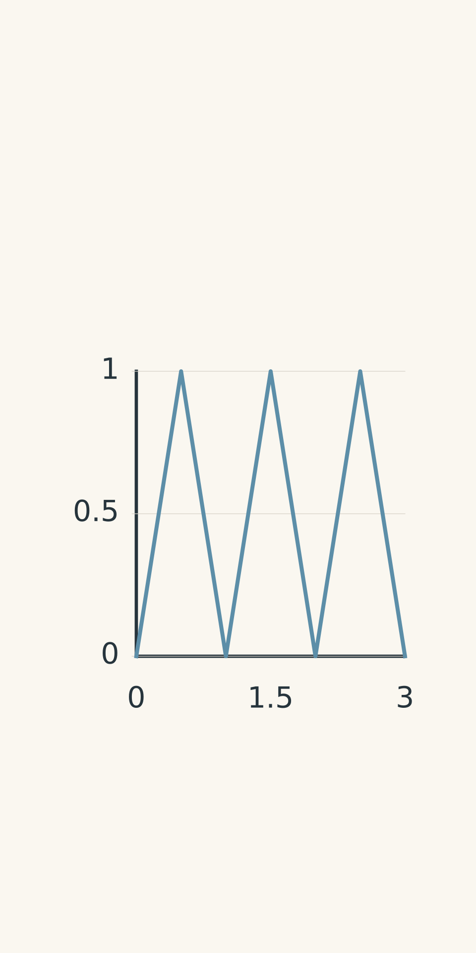
The receiver could be moved along the line where the incident and reflected waves overlapped. The positions of repeated weak responses gave information about the wavelength.
For consecutive minima in the same standing-wave pattern, the distance between them is half a wavelength.
If \(d\) is the distance between adjacent minima, then
\[ d=\frac{\lambda}{2} \]
Rearranging gives
\[ \lambda=2d \]
- Receiver response
Why is the separation half a wavelength rather than a full wavelength? The standing-wave pattern repeats after the phase relationship between the incident and reflected waves has changed through half a cycle of spatial repetition. Consequently, successive minima are separated by \(\lambda/2\).
Be careful with the first minimum. Its distance from an arbitrary reference point is not automatically half a wavelength. The reliable measurement is the separation between consecutive minima of the same response pattern.
Estimating frequency
The transmitter’s frequency was associated with its rapid electrical oscillations. It could be estimated from the electrical properties and oscillation behaviour of the source.
However, a spark-gap oscillator produces a damped burst rather than a perfectly steady sinusoidal signal. Its dominant frequency is therefore an estimate, not an exact value read directly from a modern digital frequency meter.
The crucial experimental idea is that frequency and wavelength must be determined independently. Their product can then be compared with Maxwell’s predicted speed.
If the calculated speed is close to \(3.00\times10^8\ \text{m s}^{-1}\), within the experimental uncertainty, the result supports the prediction that electromagnetic waves travel at approximately the speed of light in air.
Worked example: Calculating speed from adjacent minima
A metal reflector produces two adjacent weak-spark positions 0.42 m apart. The transmitter’s dominant frequency is estimated as \(3.50\times10^8\) Hz. Estimate the wavelength and wave speed.
Step 1: Convert the separation between minima into a wavelength.
The measured distance is half a wavelength, so
\[ \begin{aligned} \lambda&=2d\\ &=2(0.42\ \text{m})\\ &=0.84\ \text{m} \end{aligned} \]
Step 2: Use the wave equation to calculate the speed.
\[ \begin{aligned} v&=f\lambda\\ &=(3.50\times10^8\ \text{Hz})(0.84\ \text{m})\\ &=2.94\times10^8\ \text{m s}^{-1} \end{aligned} \]
Step 3: Compare the result with the predicted speed.
The calculated speed is \(2.94\times10^8\ \text{m s}^{-1}\), compared with approximately \(3.00\times10^8\ \text{m s}^{-1}\).
The result is about 2% lower than the reference value. It supports Maxwell’s prediction, although the difference and the uncertainty in the measurements should be considered before claiming exact agreement.
Worked example: Improving the wavelength estimate with repeated measurements
Four consecutive weak-spark positions are recorded at 0.12 m, 0.58 m, 1.04 m, and 1.50 m from the same reference point. The estimated frequency is \(3.25\times10^8\) Hz. Calculate the wavelength, wave speed, and percentage difference from \(3.00\times10^8\ \text{m s}^{-1}\).
Step 1: Calculate the average separation between consecutive minima.
There are four measured positions but only three intervals between them. The total distance across those intervals is
\[ 1.50-0.12=1.38\ \text{m} \]
Therefore,
\[ d=\frac{1.38\ \text{m}}{3}=0.46\ \text{m} \]
Using several intervals helps reduce the influence of uncertainty in any one position measurement.
Step 2: Calculate the wavelength.
\[ \begin{aligned} \lambda&=2d\\ &=2(0.46\ \text{m})\\ &=0.92\ \text{m} \end{aligned} \]
Step 3: Calculate the wave speed.
\[ \begin{aligned} v&=f\lambda\\ &=(3.25\times10^8\ \text{Hz})(0.92\ \text{m})\\ &=2.99\times10^8\ \text{m s}^{-1} \end{aligned} \]
Step 4: Calculate the percentage difference.
Using \(3.00\times10^8\ \text{m s}^{-1}\) as the reference speed,
\[ \begin{aligned} \text{Difference} &=\frac{|2.99-3.00|}{3.00}\times100\%\\ &\approx0.33\% \end{aligned} \]
The estimated speed is only about 0.33% below the reference value. This is consistent with Maxwell’s prediction, provided the experimental uncertainty is small enough to support the comparison.
05What Hertz’s observations did-and did not-establish
It is useful to separate three claims that are sometimes compressed into a single sentence in textbook summaries.
| Claim | Evidence from the experiments | Important limitation |
|---|---|---|
| An electrical disturbance can be detected without a connecting wire. | A spark appears in the separate receiving loop. | One spark alone does not rule out near-field coupling. |
| The disturbance behaves like a wave. | Reflection, interference patterns, and polarisation support wave behaviour. | The spark itself does not directly display the wave’s fields or measure its speed. |
| Electromagnetic waves travel at approximately the speed of light. | Independently estimated frequency and wavelength can be combined using \(v=f\lambda\). | Uncertainty in the frequency and wavelength estimates affects the calculated speed. |
There is also a historical detail worth getting right.
Introductory accounts often summarise Hertz’s work by saying that he confirmed electromagnetic waves travel at the speed of light. That captures the broad significance of his experiments, but it can make the original numerical measurement sound more precise than it was.
A later technical reassessment of Hertz’s original wavelength experiment argues that the early measurements did not provide a clean, high-precision value of \(c\). The interpretation of the standing-wave pattern and the estimated frequency of the oscillator introduced significant complications. The method of comparing \(f\lambda\) with the predicted speed is sound, but the original numerical evidence was less decisive than the simplified textbook account suggests.
IEEE Xplore
+1
For an HSC response, the key conclusion is that Hertz experimentally supported Maxwell’s prediction by generating and detecting electromagnetic waves and demonstrating their wave properties. The more precise historical point is that a receiver spark alone did not establish the wave speed, and the original speed measurement was not equivalent to a modern precision experiment.
Hertz also did not directly observe visible light emerging from his transmitter. His apparatus tested radio-frequency electromagnetic waves. The connection between those waves and visible light follows from Maxwell’s theory and the broader evidence that electromagnetic radiation shares the same fundamental wave properties.
06Questions and solutions
Question 1
An electromagnetic wave has a wavelength of 0.75 m and a frequency of \(4.0\times10^8\) Hz.
Calculate its speed and state whether the result is consistent with the predicted speed of electromagnetic waves in a vacuum.
Solution 1
The wave speed is \(3.0\times10^8\ \text{m s}^{-1}\), which matches the predicted speed of electromagnetic waves in a vacuum to the precision of the given values.
Using \(v=f\lambda\),
\[ \begin{aligned} v&=f\lambda\\ &=(4.0\times10^8\ \text{Hz})(0.75\ \text{m})\\ &=3.0\times10^8\ \text{m s}^{-1} \end{aligned} \]
The units are consistent because hertz means cycles per second, and multiplying by metres per cycle gives metres per second.
The calculated speed agrees with the predicted value. This supports the model, although a single calculation cannot establish the full experimental case for electromagnetic waves.
Question 2
A receiver loop produces a spark when placed 2 m from a spark-gap transmitter.
Explain why this observation is evidence of an electromagnetic disturbance but is not, by itself, conclusive evidence of freely propagating electromagnetic waves. Describe two further experimental tests that would strengthen the wave interpretation.
Solution 2
The receiver spark shows that an induced voltage has developed across the receiver’s gap, but it does not uniquely establish that the source has produced a freely propagating electromagnetic wave.
A rapidly changing electrical source can induce a voltage in a nearby conductor through near-field coupling. Direct detection therefore does not, on its own, distinguish this effect from a travelling wave.
Two stronger tests are:
- Reflection and interference: Introduce a metal reflector and move the receiver along the region where incident and reflected waves overlap. A regular pattern of strong and weak responses, with repeatable spacing between minima, supports the interpretation of interference between waves.
- Polarisation: Rotate the receiver loop or use an appropriate polarising arrangement. A systematic change in the detected signal with orientation supports the conclusion that the disturbance has a defined field orientation, as expected for a transverse electromagnetic wave.
The strength of the evidence comes from the combined observations. No single receiver spark is required to carry the entire argument.
Question 3
An oscillator produces electromagnetic waves in air at a frequency of \(2.0\times10^8\) Hz. Its measured wavelength is 1.5 m.
A second oscillator operates at \(3.0\times10^8\) Hz in the same medium. Assume that both waves travel at the same speed.
Predict the second wave’s wavelength and the new separation between adjacent minima in a standing-wave pattern. If an experiment instead finds that the minima separation has not changed, identify two checks that should be made before rejecting the model.
Solution 3
The second wave should have a wavelength of 1.0 m, and the separation between adjacent minima should decrease from 0.75 m to 0.50 m.
Step 1: Calculate the speed using the first oscillator.
\[ \begin{aligned} v&=f\lambda\\ &=(2.0\times10^8\ \text{Hz})(1.5\ \text{m})\\ &=3.0\times10^8\ \text{m s}^{-1} \end{aligned} \]
Step 2: Calculate the wavelength of the second wave.
Rearrange \(v=f\lambda\) to make wavelength the subject:
\[ \lambda=\frac{v}{f} \]
Substituting the second frequency,
\[ \begin{aligned} \lambda_2 &=\frac{3.0\times10^8\ \text{m s}^{-1}} {3.0\times10^8\ \text{Hz}}\\ &=1.0\ \text{m} \end{aligned} \]
The frequency has increased by a factor of 1.5, so the wavelength decreases by a factor of \(1/1.5\). Their product remains constant.
Step 3: Calculate the separation between adjacent minima.
Adjacent minima are separated by half a wavelength:
\[ d_2=\frac{\lambda_2}{2} =\frac{1.0\ \text{m}}{2} =0.50\ \text{m} \]
For the first oscillator, the separation was
\[ d_1=\frac{1.5\ \text{m}}{2} =0.75\ \text{m} \]
The predicted separation therefore decreases from 0.75 m to 0.50 m.
If the measured separation does not change, check that the two frequencies were independently estimated correctly and that the receiver is detecting the same type of minimum in both experiments. Also check the receiver’s orientation and the position measurements.
The important constraint is that, in the same medium, constant wave speed requires wavelength to vary inversely with frequency. The pattern should change when the frequency changes.
Question 4
Two groups compare the maximum distance at which a receiver produces a visible spark.
- Group A detects a spark at 5 m using a receiver gap of 0.10 mm and a loop area of \(100\ \text{cm}^2\), aligned for strong coupling.
- Group B detects a spark only up to 3 m using a receiver gap of 0.03 mm and a loop area of \(50\ \text{cm}^2\), with the loop rotated by 45 degrees.
A student concludes that Group A’s transmitter must be more powerful.
Evaluate the conclusion and describe how the experiment should be controlled to make a fair comparison.
Solution 4
The conclusion is not justified because the groups changed several properties of the receiver, so the maximum detection distance does not isolate the strength of the transmitted waves.
The narrower gap in Group B can produce a spark at a lower induced voltage, making that detector more sensitive in this respect. However, its smaller loop area and different orientation can reduce the induced response. The transmitters may also operate at different frequencies, which can affect how well a receiver responds.
A fair comparison should use the same receiver loop, gap, and orientation, and should tune the receiver appropriately for each transmitter. Both setups should be tested under the same environmental conditions, with the same measurement procedure and repeated trials.
Ideally, the experiment would also use a calibrated detector to measure the received signal rather than relying only on whether a spark appears.
A spark gap is a threshold detector, not a calibrated meter of wave strength. A visible spark tells you that the induced voltage exceeded a threshold; it does not tell you exactly how strong the incident wave was.
Question 5
A class repeats a Hertz-style experiment using two spark-gap oscillators and a metal reflector. The receiver is moved along a marked line, and weak-spark positions are recorded.
Assume that the positions in each run are consecutive minima of the same receiver response, that the listed frequencies are independently estimated, and that the standing-wave measurements are made beyond the transmitter’s immediate near field.
- Oscillator P has an estimated frequency of \(2.5\times10^8\) Hz. Three consecutive weak-spark positions are 0.20 m, 0.80 m, and 1.40 m from the chosen reference mark.
- Oscillator Q has an estimated frequency of \(4.0\times10^8\) Hz. Three consecutive weak-spark positions are 0.160 m, 0.535 m, and 0.910 m from the chosen reference mark.
In a separate check, a spark is still detected close to the transmitter when the reflector is removed. Rotating the receiver loop by 90 degrees greatly weakens this close-range response.
One student uses the first weak-spark position as \(\lambda/2\), concluding that P and Q have different wave speeds. Another argues that the close-range spark shows that all the observations could be explained by induction rather than propagating waves.
Determine the wavelength and wave speed for each oscillator. Evaluate both students’ arguments, explaining which observations are decisive and which remain ambiguous.
Hertz’s Experiment: Repeated Weak-Spark Positions
| Oscillator P | Metal reflector at one end; ruler positions measured from the reference mark. Three weak-spark markers: 0.20 m, 0.80 m, 1.40 m. Both adjacent gaps are equal: 0.60 m. |
|---|---|
| Oscillator Q | Metal reflector at one end; same ruler scale and reference convention. Three weak-spark markers: 0.160 m, 0.535 m, 0.910 m. Both adjacent gaps are equal: 0.375 m. |
Solution 5
Both oscillators give an estimated wave speed of \(3.0\times10^8\ \text{m s}^{-1}\). The first student has used the wrong distance to estimate wavelength, while the second is correct that a close-range spark alone could result from near-field coupling but is wrong to use that observation to dismiss the standing-wave evidence.
Step 1: Calculate the wavelength for oscillator P.
The consecutive minima are separated by
\[ \begin{aligned} d_P&=0.80-0.20\\ &=0.60\ \text{m} \end{aligned} \]
The next interval is also \(1.40-0.80=0.60\ \text{m}\), confirming the repeated spacing.
Since \(d_P=\lambda_P/2\),
\[ \lambda_P=2(0.60\ \text{m})=1.20\ \text{m} \]
The speed is therefore
\[ \begin{aligned} v_P&=f_P\lambda_P\\ &=(2.5\times10^8\ \text{Hz})(1.20\ \text{m})\\ &=3.0\times10^8\ \text{m s}^{-1} \end{aligned} \]
Step 2: Calculate the wavelength for oscillator Q.
The consecutive minima are separated by
\[ \begin{aligned} d_Q&=0.535-0.160\\ &=0.375\ \text{m} \end{aligned} \]
The next interval is also \(0.910-0.535=0.375\ \text{m}\).
Therefore,
\[ \lambda_Q=2(0.375\ \text{m})=0.750\ \text{m} \]
The speed is
\[ \begin{aligned} v_Q&=f_Q\lambda_Q\\ &=(4.0\times10^8\ \text{Hz})(0.750\ \text{m})\\ &=3.0\times10^8\ \text{m s}^{-1} \end{aligned} \]
Both independent estimates agree with each other and with the predicted speed to the precision of the data.
Step 3: Identify the first student’s error.
The first weak-spark position is measured from a chosen reference mark. Its distance from that mark is not automatically half a wavelength. The location of the first minimum depends on the phase relationship, the reflecting boundary, and the field component to which the receiver responds.
The spacing between consecutive minima is the reliable measurement in this problem.
If the first student incorrectly used the first position, the estimated speeds would be
\[ v_P=(2.5\times10^8)(2\times0.20) =1.0\times10^8\ \text{m s}^{-1} \]
and
\[ v_Q=(4.0\times10^8)(2\times0.160) =1.28\times10^8\ \text{m s}^{-1} \]
These values appear different, but the disagreement comes from an invalid wavelength measurement. The data themselves do not support the conclusion that the two waves travel at different speeds.
Step 4: Evaluate the induction argument.
The close-range spark without the reflector does not, by itself, rule out near-field coupling. The change in response when the loop is rotated also shows that the detector’s orientation matters, but orientation dependence alone is not conclusive evidence of freely propagating waves.
The stronger evidence is the repeating pattern of weak responses in the standing-wave measurements. The adjacent-minimum spacing changes between P and Q in the way expected when wavelength changes with frequency. Combining those independent measurements gives the same propagation speed for both oscillators.
The two students’ arguments therefore fail for different reasons. The first uses the wrong spatial measurement. The second treats a limitation of one observation as though it invalidated the entire set of observations.
The next useful connection is electromagnetic induction. The same changing fields that produce a voltage in Hertz’s receiving loop are central to how antennas receive radio signals. Understanding that connection links the historical experiment to the modern electromagnetic spectrum and the physics of wireless communication.