
Why Circuit Practical Results Differ from Ideal Calculations
Learn how to compare measured currents and potential differences with ideal circuit calculations, assess measurement uncertainties, and investigate discrepancies without assuming a single cause. Includes worked examples and five progressively challenging HSC Physics questions with detailed solutions.
You calculate a current of 25.9 mA for a combination circuit, build the circuit, and measure 25.1 mA. The difference is small, but it isn’t zero. Did you make a mistake in your calculations, connect something incorrectly, or discover that the circuit behaves differently from the model?
Before deciding, predict two things. Should the 220 Ω branch carry more or less current than the 330 Ω branch? And should the total current equal the sum of the branch currents?
Unsupported construction: circuit schematic
| Required circuit topology | A 6.0 V supply and 100 Ω resistor in series with parallel 220 Ω and 330 Ω branches must be drawn as connected electrical components. The requested wire paths, current arrows, and voltage-measurement points cannot be represented by this schema. |
|---|---|
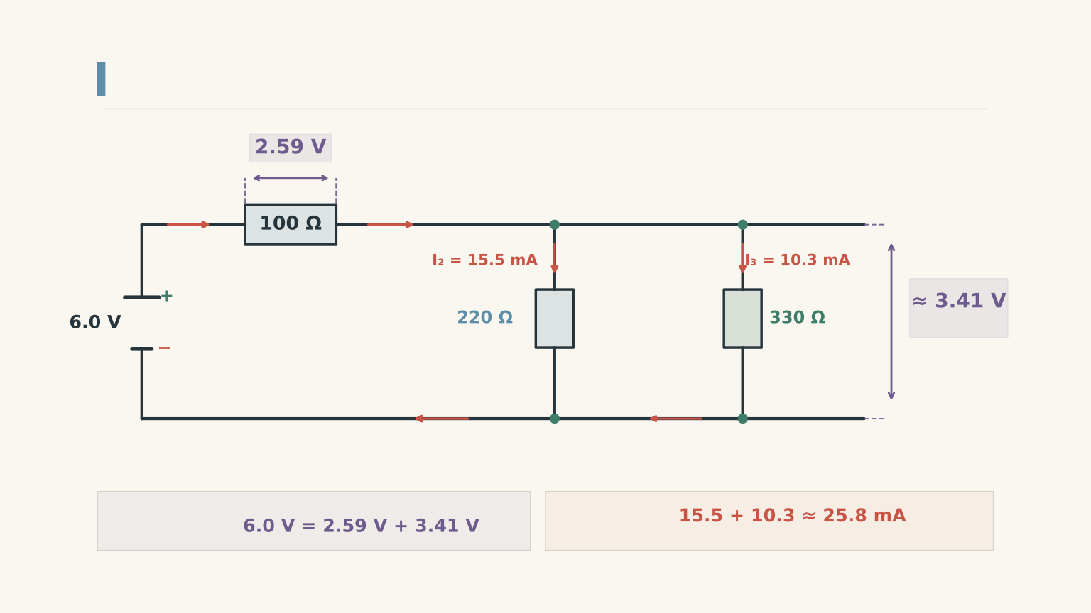
| Scientific relationships to preserve | Iₜ = I₂₂₀ + I₃₃₀ The 220 Ω branch carries more current than the 330 Ω branch. Ideal total current is 25.9 mA; the voltage across both parallel branches is approximately 3.41 V. |
The 220 Ω branch should carry more current because its resistance is lower. The total current should also equal the sum of the two branch currents because charge cannot disappear at a junction.
Those predictions are more useful than immediately blaming your equipment. They give you relationships to test against your measurements, even when the exact values differ from your calculations.
01Start with what the circuit should do
Before analysing practical results, make sure you can predict the behaviour of the ideal circuit. This is the reference model you’ll compare your measurements against.
Series and parallel circuits
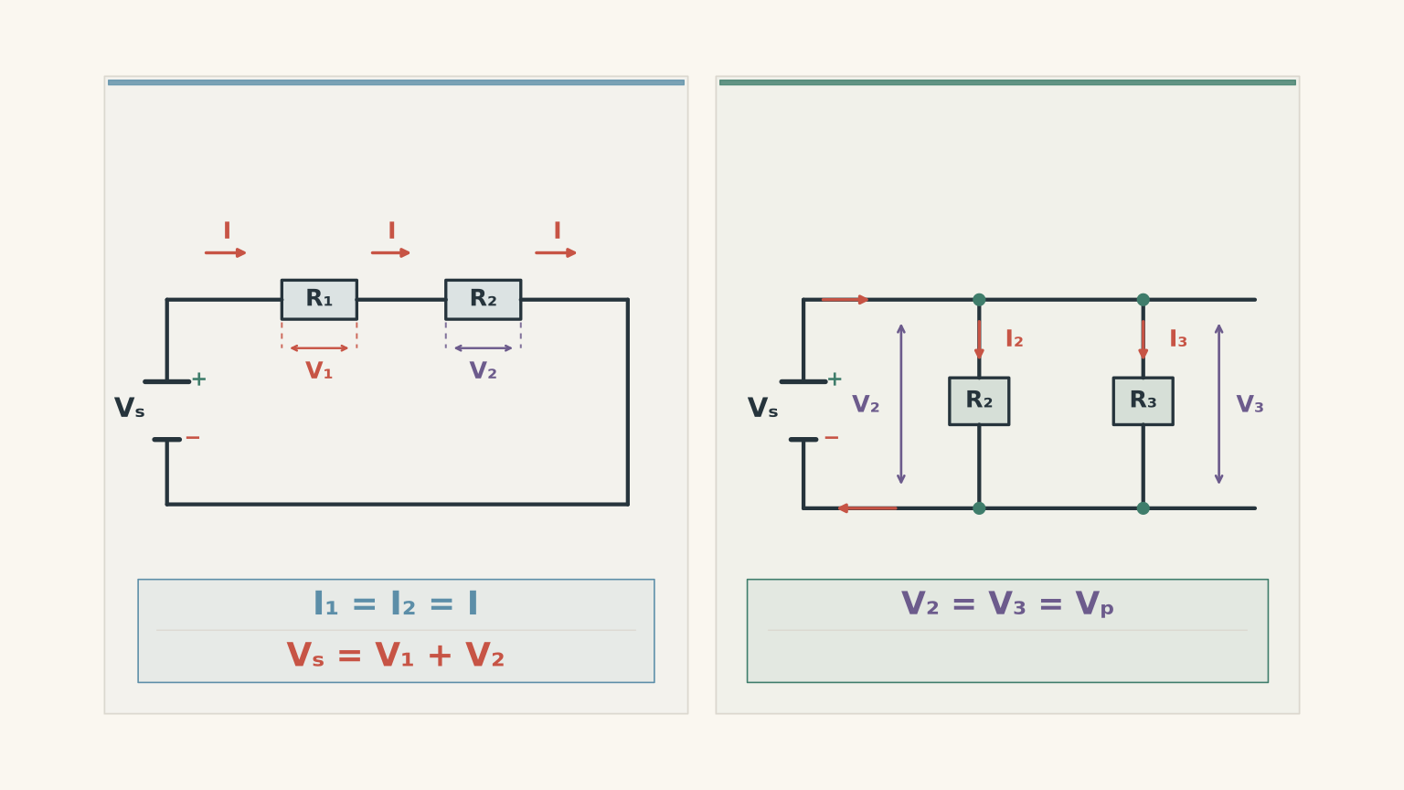
In a series circuit, components are connected along the same path. The same current passes through each component, while the supply potential difference is shared between them.
For a loop containing two resistors,
\[ I_1=I_2=I \]
and
\[ V_s=V_1+V_2 \]
Here, \(I\) represents current, \(V\) represents potential difference, and the subscripts identify the component or supply being measured.
In a parallel circuit, branches connect between the same two electrical nodes. A node is a connection point shared by circuit components.
Each branch has the same potential difference across it, but the current can differ between branches.
\[ V_2=V_3=V_p \]
At the junction, the current divides and later recombines:
\[ I_{\text{total}}=I_2+I_3 \]
Think of two routes between the same starting point and destination. More flow can pass through the easier route, but the flow doesn’t vanish when the routes split.
The analogy has a limit: electrical current isn’t a crowd choosing where to walk. Its distribution is determined by the potential difference and the resistance of each branch.
For an ordinary resistor at constant temperature, Ohm’s law gives the relationship between these quantities:
\[ V=IR \]
where \(V\) is the potential difference in volts, \(I\) is the current in amperes, and \(R\) is the resistance in ohms.
For two parallel resistors, the equivalent resistance is
\[ R_p=\frac{R_2R_3}{R_2+R_3} \]
The equivalent resistance is smaller than either individual resistance. Adding a parallel path makes it easier for current to flow through the combination.
These relationships give you a starting point for calculating the expected current and potential differences.
Worked example: Predict the currents and voltages
A 6.0 V ideal supply is connected to a 100 Ω resistor in series with a parallel combination of 220 Ω and 330 Ω resistors. Calculate the total current, the potential difference across each section, and the current through each parallel branch.
Assume the supply maintains exactly 6.0 V and all resistors have their stated values.
Step 1
\[ \begin{aligned} R_p&=\frac{220\times330}{220+330}\\ &=\frac{72600}{550}\\ &=132\ \Omega \end{aligned} \]
Step 2
\[ R_{\text{total}}=100+132=232\ \Omega \]
Step 3
\[ \begin{aligned} I_{\text{total}}&=\frac{V_s}{R_{\text{total}}}\\ &=\frac{6.0}{232}\\ &=0.02586\ \text{A}\\ &=25.9\ \text{mA} \end{aligned} \]
The supply current is approximately 25.9 mA. Because the 100 Ω resistor is in series with the parallel section, this same current passes through the 100 Ω resistor.
Step 4
\[ \begin{aligned} V_{100}&=IR\\ &=0.02586\times100\\ &=2.59\ \text{V} \end{aligned} \]
The remaining potential difference is across the parallel section:
\[ V_p=6.0-2.59=3.41\ \text{V} \]
Both parallel resistors have approximately 3.41 V across them.
Step 5
For the 220 Ω resistor,
\[ I_{220}=\frac{3.41}{220} \approx15.5\ \text{mA} \]
For the 330 Ω resistor,
\[ I_{330}=\frac{3.41}{330} \approx10.3\ \text{mA} \]
Step 6
\[ 15.5+10.3=25.8\ \text{mA} \]
The small difference between 25.8 mA and 25.9 mA comes from rounding. Before rounding, the branch currents add to the total current.
This calculation gives you two different things to check in a practical: whether the measured values are close to the predictions, and whether the measured values obey the circuit relationships.
Those are not the same test.
02Why practical results differ from ideal calculations
An ideal circuit assumes that the supply voltage and component resistances are known exactly, the connecting wires have zero resistance, and the measuring instruments do not affect the circuit.
A real practical doesn’t satisfy all those assumptions perfectly.
The important distinction is between a difference in the numerical values and a failure of a relationship.
For example, a resistor marked 220 Ω might actually have a resistance of 226 Ω. Your calculation using 220 Ω would then give an approximate prediction, but the actual circuit can still obey Ohm’s law and Kirchhoff’s laws.
By contrast, if the measured total current differs substantially from the sum of the branch currents, changing a resistor’s value doesn’t explain that discrepancy. You need to investigate the measurements, connections, or conditions under which they were taken.
Measurement resolution is not the same as accuracy
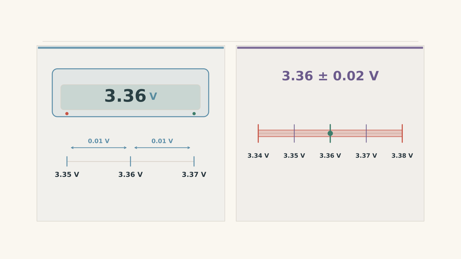
Suppose a digital voltmeter displays 3.36 V.
Its resolution might be 0.01 V, meaning its display changes in increments of 0.01 V on that range. This does not automatically mean that the true voltage is within 0.01 V of the displayed value.
Accuracy describes how close the reading is to the actual value. The instrument’s stated accuracy, calibration, range, and operating conditions affect how much confidence you can place in the reading.
The uncertainty is the range you reasonably associate with a measurement.
For example, if a practical specifies a reading of \(3.36\pm0.02\text{ V}\), the stated uncertainty is ±0.02 V. Use the uncertainty supplied by the experiment or the instrument specifications rather than assuming that the final displayed digit tells you everything.
When comparing two measurements, compare the size of their discrepancy with the uncertainties involved.
For a simple school-level check, adding the absolute uncertainties of the readings being compared gives a conservative estimate. Follow your practical instructions if a more formal uncertainty calculation is required.
A discrepancy smaller than the combined uncertainty may be consistent with measurement limitations. A discrepancy substantially larger than the combined uncertainty needs investigation.
Neither result identifies the cause by itself.
Worked example: Are the measured values consistent?
You build the same circuit from the previous example. The supply is measured at 5.94 V while the circuit is operating, rather than the nominal 6.0 V.
The resistors are marked with a tolerance of ±5%. Your recorded readings are:
| Quantity | Measured value |
|---|---|
| Supply potential difference | \(5.94\pm0.02\text{ V}\) |
| Potential difference across 100 Ω | \(2.56\pm0.02\text{ V}\) |
| Potential difference across 220 Ω | \(3.36\pm0.02\text{ V}\) |
| Potential difference across 330 Ω | \(3.37\pm0.02\text{ V}\) |
| Total current | \(25.3\pm0.2\text{ mA}\) |
| Current through 220 Ω | \(15.2\pm0.2\text{ mA}\) |
| Current through 330 Ω | \(10.0\pm0.2\text{ mA}\) |
Assess whether the readings are consistent with the circuit rules and compare them with the ideal predictions.
Step 1
The equivalent resistance, using the marked resistor values, remains
\[ R_{\text{total}}=232\ \Omega \]
Therefore,
\[ \begin{aligned} I_{\text{predicted}}&=\frac{5.94}{232}\\ &=0.02560\ \text{A}\\ &=25.6\ \text{mA} \end{aligned} \]
The predicted potential differences are
\[ \begin{aligned} V_{100}&=0.02560\times100\\ &\approx2.56\ \text{V}\\[4pt] V_p&=5.94-2.56\\ &\approx3.38\ \text{V} \end{aligned} \]
The predicted branch currents are approximately 15.4 mA through the 220 Ω resistor and 10.2 mA through the 330 Ω resistor.
Step 2
Using the readings for the 100 Ω and 220 Ω resistors,
\[ 2.56+3.36=5.92\ \text{V} \]
The measured supply voltage is 5.94 V, giving a difference of 0.02 V.
The conservative combined uncertainty is
\[ 0.02+0.02+0.02=0.06\ \text{V} \]
The discrepancy of 0.02 V is smaller than this uncertainty. The voltage readings are therefore consistent with the loop relationship.
Using the 330 Ω branch gives \(2.56+3.37=5.93\text{ V}\), which is also consistent.
Step 3
The measured branch voltages differ by
\[ |3.36-3.37|=0.01\ \text{V} \]
The combined uncertainty of these two readings is 0.04 V using the conservative method. Their difference is smaller than that uncertainty.
The readings are consistent with the branches having the same potential difference.
Step 4
The measured branch currents add to
\[ I_{\text{branches}}=15.2+10.0=25.2\ \text{mA} \]
The total current is 25.3 mA, giving a discrepancy of
\[ |25.3-25.2|=0.1\ \text{mA} \]
The conservative combined uncertainty is
\[ 0.2+0.2+0.2=0.6\ \text{mA} \]
The discrepancy is smaller than the combined uncertainty. The current readings are consistent with Kirchhoff’s current law.
Step 5
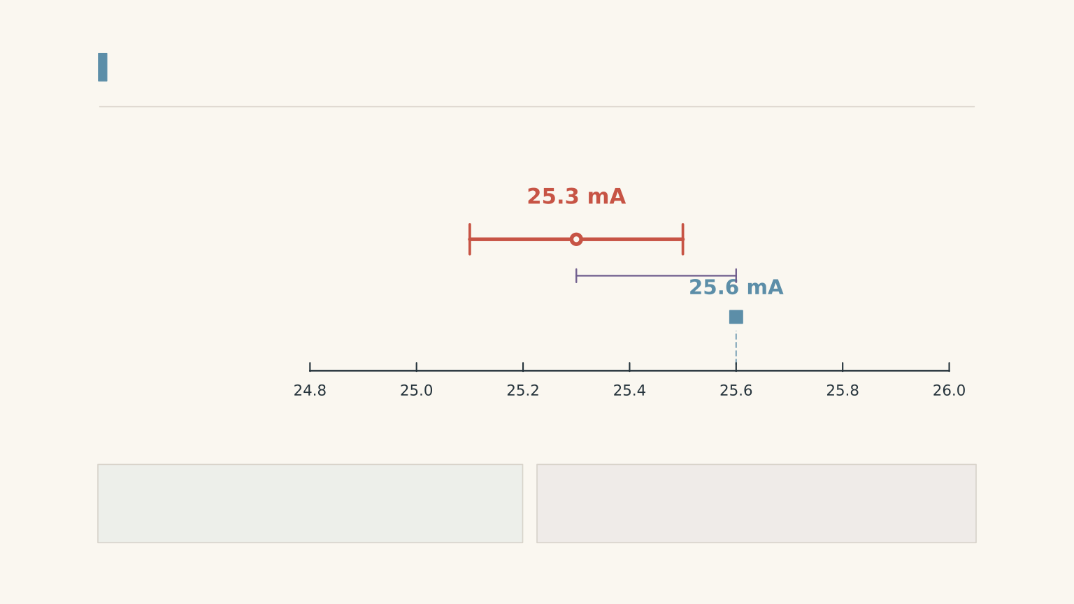
The measured total current is 25.3 mA, compared with a nominal-value prediction of 25.6 mA. That difference is 0.3 mA.
The stated current measurement uncertainty alone does not fully account for the difference. However, the ±5% resistor tolerance means the actual resistance values can differ from the marked values. The nominal calculation is not an exact prediction of the real circuit.
The voltage and current relationships are consistent within the stated measurement uncertainties. The small difference from the nominal predictions does not establish a fault, and the readings do not identify a single cause.
03Five plausible causes of discrepancies
A useful investigation looks for a cause that fits the pattern of the results. Don’t decide in advance that every discrepancy must come from the same source.
1. Resistor tolerance
A resistor marked 220 Ω may not have an actual resistance of exactly 220 Ω. Its permitted tolerance describes the range of resistance values around its nominal value.
If the actual resistance is higher than the marked value, the current through that resistor will generally be lower than a calculation using the nominal resistance predicts, assuming the potential difference is unchanged.
Tolerance affects the numerical predictions. It does not remove the requirement for current to be conserved at a junction.
To investigate, measure the resistance with the circuit switched off and the resistor isolated from other current paths. In-circuit resistance measurements can be affected by other components connected across the same nodes.
2. The supply voltage changes under load
A power supply or battery may have a different terminal voltage when current is flowing than when the circuit is disconnected.
A simple model represents a source as an ideal electromotive force, \(\mathcal{E}\), in series with an internal resistance, \(r\). The terminal potential difference while current flows is
\[ V_{\text{terminal}}=\mathcal{E}-Ir \]
Here, \(I\) is the current supplied by the source.
The internal resistance causes a potential difference inside the source. Consequently, the voltage available to the external circuit can be lower than the open-circuit voltage.
A regulated bench supply may show very little change under normal loading, while a battery or a supply approaching its current limit may behave differently.
Measure the supply voltage while the circuit is operating. Don’t automatically use the voltage printed on a battery or the nominal setting of a power supply as the actual voltage across the connected circuit.
3. Measuring instruments affect the circuit
An ideal ammeter has zero resistance. You connect it in series so the current flowing through the component also flows through the meter.
A real ammeter has some internal resistance and may introduce a small additional potential difference, sometimes described as its burden voltage. This can reduce the current compared with the ideal prediction.
An ideal voltmeter has infinite resistance, so no current flows through it. A real voltmeter has a finite input resistance and draws some current.
When you connect a voltmeter across a resistor, the meter creates an additional parallel path. If its input resistance is not sufficiently high compared with the resistor, it can change the circuit’s equivalent resistance.
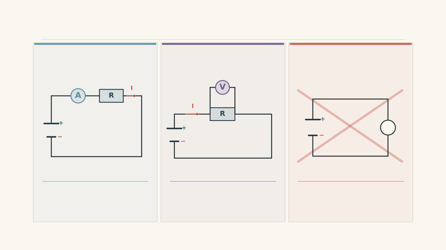
The size of these effects depends on the actual instrument and circuit. Many digital voltmeters have sufficiently high input resistance that their effect is negligible in ordinary resistor circuits, but you should check the specifications rather than assume this.
Also consider how you measured the current. If you move an ammeter from the main circuit into a branch, its added resistance may change the circuit. Readings taken in different configurations might not add up exactly, even if each individual reading is reasonable.
4. Connections and wiring
A loose connection or a poor contact can add resistance to a circuit. This can change the current and the potential difference across individual components.
Incorrect meter placement can cause a different problem. A voltmeter connected to the wrong pair of nodes may measure the potential difference across a component plus a connecting lead or contact, rather than across the component alone.
If two supposed parallel branches appear to have substantially different potential differences, first check that both measurements were made across the same two nodes.
A wiring problem is one possibility, not an automatic diagnosis. Verify the circuit before replacing components or changing your calculations.
5. Temperature and component behaviour
The resistance of a component can change as it heats up. For many fixed resistors, this effect is relatively small under normal operating conditions, but it depends on the component and its temperature.
A filament lamp is a more obvious example. Its filament has a much lower resistance when cold than when hot. As the lamp warms, its resistance rises, so its current does not follow the simple prediction you would make using its cold resistance.
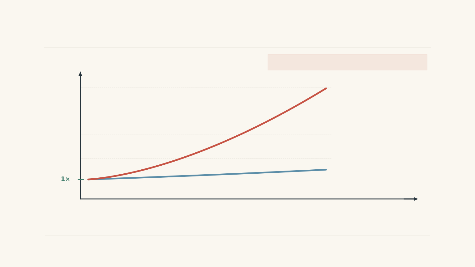
This creates an important experimental issue: the circuit may change while you’re measuring it.
If you record the total current immediately after switching on, then record branch currents after a lamp has warmed, those readings describe different circuit states. They should not be combined as though they were measured simultaneously under identical conditions.
04A practical method for investigating your results
When your measured values differ from your calculations, use a consistent sequence. It prevents you from spending time investigating a cause that the evidence doesn’t support.
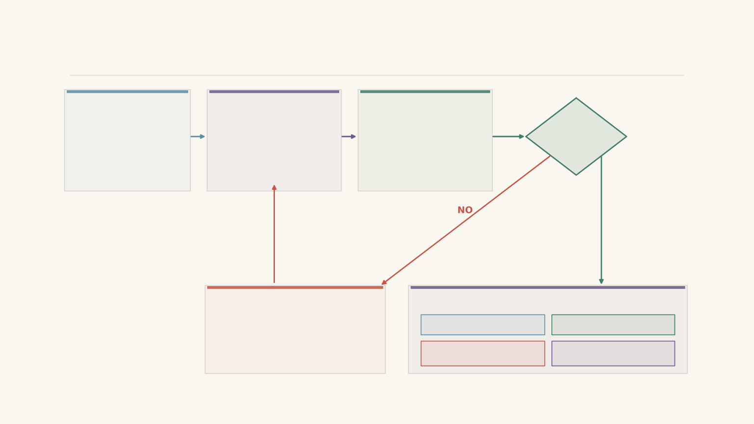
Step 1: Record the circuit conditions
Before switching on, note the marked resistance of each component, its tolerance if available, the supply setting, and the meter ranges.
Record whether a component was cold, warming, or at a steady operating temperature. If the supply voltage changes under load, record the loaded value as well.
Step 2: Check the meter connections
Confirm that the ammeter is in series with the intended current path and that the voltmeter is connected across the intended component.
Check the polarity and range. Switch off the supply before changing connections, and never connect an ammeter directly across the supply.
Step 3: Compare the measured values with the predictions
Use the actual measured supply voltage where possible, rather than relying only on its nominal value.
Calculate the predicted current and potential differences using the marked resistor values. Report sensible significant figures and keep the measured values separate from the calculated values.
Step 4: Test the circuit relationships
For a junction, calculate the difference between the measured total current and the sum of the measured branch currents:
\[ \Delta I= \left|I_{\text{total}}-\sum I_{\text{branches}}\right| \]
For a loop, compare the measured supply potential difference with the sum of the potential differences across the external components:
\[ \Delta V= \left|V_s-\sum V_{\text{drops}}\right| \]
Compare these discrepancies with the uncertainties of the readings involved.
If the discrepancy is small enough to be consistent with the uncertainties, report that result. If it is too large, investigate the measurements and circuit configuration before claiming that a particular component is responsible.
Remember that the external voltage drops should add to the source’s terminal voltage. If you use the source’s electromotive force instead, account for the potential difference across its internal resistance.
Step 5: Test one plausible explanation at a time
Use the pattern of the discrepancy to decide what to check next.
| Observation | Useful checks |
|---|---|
| The measured current is lower than predicted. | Check the loaded supply voltage, actual resistance, and ammeter resistance. |
| Parallel branch voltages differ beyond their uncertainties. | Check that the voltmeter is connected across the same two nodes in each measurement. |
| The total current does not match the branch-current sum. | Check current-meter placement, the measurement sequence, possible unmeasured branches, and whether readings represent the same circuit state. |
| The measured values change as time passes. | Check whether components are heating or the supply is changing under load. |
| Voltage drops do not add to the measured supply voltage within uncertainty. | Check the measurement points, readings, connections, and whether all values were recorded under the same conditions. |
These are starting points for an investigation, not one-to-one diagnoses. Several effects can occur at once.
05Questions and solutions
Question 1
A 9.0 V ideal supply is connected to a 150 Ω resistor in series with parallel 300 Ω and 600 Ω resistors.
Calculate the total resistance, the total current, the potential difference across the parallel section, and the current through each parallel branch.
Solution 1
The total resistance is 350 Ω, the total current is 25.7 mA, and the two branch currents are 17.1 mA and 8.57 mA. These results follow from combining the parallel resistors first, then treating the equivalent resistance as a series component.
Step 1: Calculate the parallel equivalent resistance.
\[ \begin{aligned} R_p&=\frac{300\times600}{300+600}\\ &=\frac{180000}{900}\\ &=200\ \Omega \end{aligned} \]
Step 2: Calculate the total resistance and current.
\[ R_{\text{total}}=150+200=350\ \Omega \]
\[ \begin{aligned} I_{\text{total}}&=\frac{9.0}{350}\\ &=0.0257\ \text{A}\\ &=25.7\ \text{mA} \end{aligned} \]
Step 3: Find the potential difference across the parallel section.
The potential difference across the 150 Ω resistor is
\[ V_{150}=0.0257\times150=3.86\ \text{V} \]
Therefore,
\[ V_p=9.0-3.86=5.14\ \text{V} \]
Step 4: Calculate the branch currents.
For the 300 Ω resistor,
\[ I_{300}=\frac{5.14}{300}=17.1\ \text{mA} \]
For the 600 Ω resistor,
\[ I_{600}=\frac{5.14}{600}=8.57\ \text{mA} \]
The currents add to approximately 25.7 mA. The lower-resistance branch carries more current, while both branches have the same potential difference.
Question 2
A circuit contains a 100 Ω resistor in series with parallel 220 Ω and 330 Ω resistors. During a practical, the following readings are recorded. Each uncertainty is supplied by the experimental setup.
| Quantity | Reading |
|---|---|
| Supply voltage | \(6.00\pm0.02\text{ V}\) |
| Voltage across 100 Ω | \(2.59\pm0.02\text{ V}\) |
| Voltage across 220 Ω | \(3.40\pm0.02\text{ V}\) |
| Voltage across 330 Ω | \(3.39\pm0.02\text{ V}\) |
| Total current | \(25.4\pm0.2\text{ mA}\) |
| Current through 220 Ω | \(15.4\pm0.2\text{ mA}\) |
| Current through 330 Ω | \(8.8\pm0.2\text{ mA}\) |
Assume the resistors have a tolerance of ±5%. Determine which circuit relationships are consistent with the readings. Can resistor tolerance alone explain the current discrepancy? State what you would investigate first.
Solution 2
The voltage readings are consistent with the series-loop and parallel-branch relationships, but the measured currents are not consistent with current conservation at the junction. Resistor tolerance alone cannot explain the current discrepancy.
Step 1: Check the parallel voltages.
Their difference is
\[ |3.40-3.39|=0.01\ \text{V} \]
The combined uncertainty is 0.04 V using the conservative method. The difference is within this uncertainty, so the readings are consistent with equal potential differences across the parallel branches.
Step 2: Check the loop potential differences.
Using the 220 Ω branch,
\[ 2.59+3.40=5.99\ \text{V} \]
The measured supply voltage is 6.00 V, so the discrepancy is 0.01 V.
The conservative combined uncertainty is 0.06 V, making the readings consistent with the loop relationship.
Using the 330 Ω branch gives 5.98 V, which is also consistent.
Step 3: Check the junction current.
The branch currents add to
\[ I_{\text{branches}}=15.4+8.8=24.2\ \text{mA} \]
The measured total current is 25.4 mA. The discrepancy is
\[ \Delta I=|25.4-24.2|=1.2\ \text{mA} \]
The conservative combined uncertainty is
\[ 0.2+0.2+0.2=0.6\ \text{mA} \]
The discrepancy exceeds the combined uncertainty, so the current readings are not consistent with the junction relationship.
Step 4: Explain why resistor tolerance is not enough.
Resistor tolerance can change the predicted current through each branch. However, in a single unchanged circuit, the total current entering the junction must still equal the sum of the currents leaving it.
The measured voltage across the 330 Ω resistor also suggests a current of approximately
\[ I_{330}=\frac{3.39}{330} \approx10.3\ \text{mA} \]
This is noticeably higher than the recorded 8.8 mA. The difference warrants checking the branch-current measurement, although the calculation uses the nominal resistance.
First, check the ammeter’s connection and range, confirm that the correct branch was measured, and verify that the readings were taken under comparable conditions. If the ammeter was moved between the main circuit and a branch, its resistance may have changed the circuit slightly between readings.
The evidence identifies an inconsistency, not a unique cause. It does not prove that the ammeter itself is faulty.
Question 3
A 6.0 V ideal supply drives a 100 Ω resistor in series with parallel 220 Ω and 330 Ω resistors.
An ideal voltmeter would have infinite input resistance. Instead, a voltmeter with an input resistance of 10.0 kΩ is connected across the 220 Ω resistor.
Assuming all other components and the ammeter are ideal, calculate the new total current. Explain why it differs from the prediction made with an ideal voltmeter.
Solution 3
The total current increases from approximately 25.9 mA to 26.1 mA because the voltmeter provides an additional parallel current path, reducing the equivalent resistance of the circuit.
Step 1: Calculate the original total current.
Without the voltmeter affecting the circuit,
\[ R_p=\frac{220\times330}{220+330} =132\ \Omega \]
Thus,
\[ R_{\text{total}}=100+132=232\ \Omega \]
and
\[ I_{\text{total}}=\frac{6.0}{232} =25.9\ \text{mA} \]
Step 2: Include the voltmeter’s input resistance.
The voltmeter is connected in parallel with the 220 Ω resistor. Their equivalent resistance is
\[ \begin{aligned} R_{220,m} &=\frac{220\times10000}{220+10000}\\ &\approx215.3\ \Omega \end{aligned} \]
This is slightly lower than 220 Ω.
Step 3: Calculate the new parallel and total resistances.
The effective parallel resistance is now
\[ R_p=\frac{215.3\times330}{215.3+330} \approx130.3\ \Omega \]
Adding the 100 Ω series resistor gives
\[ R_{\text{total}}=100+130.3=230.3\ \Omega \]
Step 4: Calculate the new total current.
\[ \begin{aligned} I_{\text{total}}&=\frac{6.0}{230.3}\\ &=0.0261\ \text{A}\\ &=26.1\ \text{mA} \end{aligned} \]
The current increases because the effective resistance decreases. Some current now flows through the voltmeter as well as through the 220 Ω resistor.
This example deliberately uses a relatively low voltmeter input resistance to make the effect visible. A meter with a much higher input resistance would produce a much smaller change.
Question 4
A battery has an electromotive force of 6.00 V and an internal resistance of 8.0 Ω. It supplies the circuit consisting of a 100 Ω resistor in series with parallel 220 Ω and 330 Ω resistors.
Assume all resistances remain constant and the meters are ideal.
Calculate the total current, the battery’s terminal voltage while supplying the circuit, the potential difference across the 100 Ω resistor, and the current through each parallel branch. Explain why the battery’s open-circuit voltage is not the correct potential difference to use across the external circuit.
Solution 4
The total current is 25.0 mA, and the loaded terminal voltage is 5.80 V. The internal resistance accounts for the 0.20 V difference between the battery’s electromotive force and its terminal voltage.
Step 1: Calculate the external resistance.
The parallel section has an equivalent resistance of 132 Ω, so
\[ R_{\text{external}}=100+132=232\ \Omega \]
Step 2: Include the internal resistance.
The total resistance in the complete loop is
\[ R_{\text{loop}}=232+8.0=240\ \Omega \]
Therefore,
\[ \begin{aligned} I&=\frac{\mathcal{E}}{R_{\text{loop}}}\\ &=\frac{6.00}{240}\\ &=0.0250\ \text{A}\\ &=25.0\ \text{mA} \end{aligned} \]
Step 3: Calculate the terminal voltage.
The potential difference across the internal resistance is
\[ V_r=Ir=0.0250\times8.0=0.20\ \text{V} \]
Hence,
\[ V_{\text{terminal}}=6.00-0.20=5.80\ \text{V} \]
This is the potential difference available across the external circuit while current is flowing.
Step 4: Calculate the external potential differences.
Across the 100 Ω resistor,
\[ V_{100}=0.0250\times100=2.50\ \text{V} \]
Across the parallel section,
\[ V_p=5.80-2.50=3.30\ \text{V} \]
Step 5: Calculate the branch currents.
\[ I_{220}=\frac{3.30}{220}=15.0\ \text{mA} \]
\[ I_{330}=\frac{3.30}{330}=10.0\ \text{mA} \]
The branch currents add to 25.0 mA, as required.
The tempting mistake is to assume that a battery labelled 6.00 V always provides 6.00 V across the external circuit. With internal resistance, some of the electromotive force is associated with a potential drop inside the battery while current flows. The open-circuit reading can therefore differ from the loaded terminal voltage.
Question 5
A 6.00 V source has an internal resistance of 10.0 Ω. It is connected to a 100 Ω resistor in series with a parallel combination of a 220 Ω fixed resistor and a filament lamp.
The lamp has a resistance of 30 Ω immediately after switching on and a resistance of 120 Ω once it has warmed up. Assume these resistance values remain constant during their respective calculations, and treat the source and all other components as ideal apart from the stated internal resistance.
A student records the total current immediately after switching on, then measures the branch currents after the lamp has warmed up. The student argues:
- The lamp’s resistance has increased, so its potential difference must have decreased.
- The later branch currents do not add to the earlier total current, so current must have been lost somewhere in the circuit.
Calculate the total current, the potential difference across the parallel section, and both branch currents in the cold and warm states. Evaluate both claims.
Solution 5
Both claims are incorrect. The total current falls from approximately 44.0 mA to 32.0 mA as the lamp warms, but the potential difference across the parallel section rises from approximately 1.16 V to 2.48 V. The apparent failure of current conservation occurs because the student is comparing measurements taken in different circuit states.
Step 1: Calculate the cold lamp’s parallel resistance.
Immediately after switching on, the lamp has a resistance of 30 Ω.
\[ \begin{aligned} R_{p,\text{cold}} &=\frac{30\times220}{30+220}\\ &=26.4\ \Omega \end{aligned} \]
The complete loop includes the 100 Ω resistor and the source’s 10.0 Ω internal resistance:
\[ R_{\text{loop,cold}}=100+10.0+26.4 =136.4\ \Omega \]
Step 2: Calculate the cold-state total current and branch voltage.
\[ \begin{aligned} I_{\text{cold}}&=\frac{6.00}{136.4}\\ &=0.04399\ \text{A}\\ &\approx44.0\ \text{mA} \end{aligned} \]
The potential difference across the parallel section is
\[ \begin{aligned} V_{p,\text{cold}} &=I_{\text{cold}}\times26.4\\ &\approx1.16\ \text{V} \end{aligned} \]
Step 3: Calculate the cold-state branch currents.
The lamp current is
\[ I_{\text{lamp,cold}}=\frac{1.16}{30} \approx38.7\ \text{mA} \]
The current through the fixed resistor is
\[ I_{220,\text{cold}}=\frac{1.16}{220} \approx5.28\ \text{mA} \]
The two branch currents add to approximately 44.0 mA, matching the total current in the cold state.
Step 4: Recalculate the circuit when the lamp is warm.
The lamp resistance is now 120 Ω, so the parallel equivalent resistance becomes
\[ \begin{aligned} R_{p,\text{warm}} &=\frac{120\times220}{120+220}\\ &\approx77.65\ \Omega \end{aligned} \]
The total loop resistance is
\[ R_{\text{loop,warm}}=100+10.0+77.65 =187.65\ \Omega \]
The warm-state total current is
\[ \begin{aligned} I_{\text{warm}}&=\frac{6.00}{187.65}\\ &\approx0.03197\ \text{A}\\ &\approx32.0\ \text{mA} \end{aligned} \]
The total current has decreased because the equivalent resistance of the complete circuit has increased.
Step 5: Calculate the warm-state potential difference and branch currents.
The potential difference across the parallel section is
\[ \begin{aligned} V_{p,\text{warm}} &=I_{\text{warm}}\times77.65\\ &\approx2.48\ \text{V} \end{aligned} \]
The lamp current is now
\[ I_{\text{lamp,warm}}=\frac{2.48}{120} \approx20.7\ \text{mA} \]
The current through the fixed resistor is
\[ I_{220,\text{warm}}=\frac{2.48}{220} \approx11.3\ \text{mA} \]
The branch currents add to approximately 32.0 mA, matching the warm-state total current.
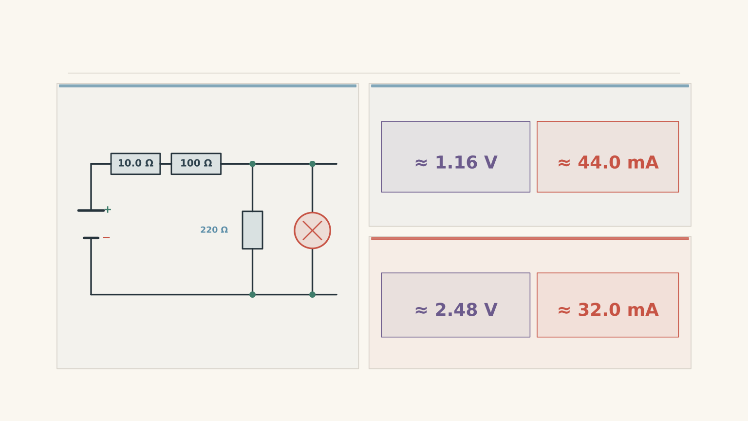
Step 6: Explain why the lamp’s potential difference rises as it warms.
The lamp’s potential difference is not fixed at the supply voltage. It depends on how the source voltage is shared between the series components and the parallel section.
When the lamp warms, the equivalent resistance of the parallel section increases. The total circuit current falls, so the potential difference across the 100 Ω series resistor decreases. The potential drop across the source’s internal resistance also decreases.
As a result, more of the source’s electromotive force is available across the parallel section. The lamp’s potential difference rises even though its current falls.
The lamp’s increasing resistance is still consistent with Ohm’s law at each state. Its current depends on both its resistance and the potential difference across it, and both quantities have changed.
Step 7: Explain why the current readings do not violate current conservation.
The cold-state total current is approximately 44.0 mA, and the cold branch currents add to approximately 44.0 mA.
The warm-state total current is approximately 32.0 mA, and the warm branch currents add to approximately 32.0 mA.
The student’s apparent discrepancy comes from comparing the cold-state total current with the warm-state branch currents. Those readings describe different conditions, so they cannot be combined in a single current-conservation check.
The next useful step in a circuit practical is to record the state of the circuit alongside every measurement, then test the current and voltage relationships before investigating possible causes. Once those checks are consistent, you can compare the results with a more realistic model that includes resistance tolerance, meter loading, internal resistance, and temperature.