
Projectile Motion Assumptions in HSC Physics Explained
Learn why HSC projectile motion assumes constant gravity and negligible air resistance, how those assumptions shape the equations, and when the model breaks down.
A calculator can be perfectly right and still predict the wrong landing point. Launch a ball, use the projectile equations, and you might calculate a range of 50 m. In the real world, the ball may land several metres short.
So which part failed: the algebra, the equation, or the model underneath it?
Before reading on, make a prediction. If you launch the same ball much faster, will the simple projectile model usually become more accurate or less accurate? For an object moving through air, usually less accurate. The faster it moves, the more important air resistance tends to become.
That is the point of projectile motion assumptions. The equations are not claiming that real projectiles literally experience constant gravity and zero air resistance. They are describing a simplified physical model. Your job in HSC Physics is to know what that model predicts, why it works so well in many situations, and when you should stop trusting it.
01What the standard projectile model is assuming
Once an object has been launched and is no longer being pushed by the launcher, the simplest model says that gravity is the only significant force acting on it.
That gives us two major assumptions:
| Assumption | What it means physically | Mathematical consequence |
|---|---|---|
| Gravity is constant | The gravitational acceleration has essentially constant magnitude and direction during the flight | \(a_y=-g\), where \(g\approx9.8\text{ m s}^{-2}\) near Earth’s surface |
| Air resistance is negligible | Forces from the surrounding air are small enough to ignore | \(a_x=0\), so horizontal velocity stays constant |
We also normally treat the ground as locally flat and the projectile as a particle whose size does not matter.
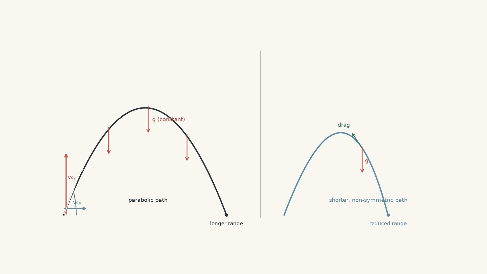
These assumptions are what make the familiar projectile equations possible. Remove them, and the equations may no longer describe the motion.
02Build the model from two motions happening at once
Imagine filming a projectile and marking its position every 0.1 s.
Horizontally, the marks would be equally spaced if there were no air resistance. That tells us the horizontal velocity is constant.
Vertically, the spacing changes because gravity continually changes the vertical velocity.
The useful trick is to treat these as two components of one motion:
- horizontal motion with zero acceleration,
- vertical motion with constant downward acceleration.
They share the same clock. If the projectile has been moving for 2 s horizontally, it has also been falling under gravity for exactly 2 s vertically.
It is a little like two students doing different subjects during the same exam period. One is doing Maths and one is doing Physics, so their work develops differently, but the clock on the wall is the same for both. The analogy breaks because the two motions are not genuinely separate objects; they are components of one velocity vector.
Suppose a projectile is launched with speed \(u\) at an angle \(\theta\) above the horizontal. Its initial velocity components are
\[
u_x=u\cos\theta
\]
and
\[
u_y=u\sin\theta
\]
where:
- \(u\) is the launch speed in \(\text{m s}^{-1}\),
- \(u_x\) is the initial horizontal velocity in \(\text{m s}^{-1}\),
- \(u_y\) is the initial vertical velocity in \(\text{m s}^{-1}\),
- \(\theta\) is the launch angle above the horizontal.
Under the standard model,
\[
a_x=0
\]
and
\[
a_y=-g
\]
if upward is taken as positive.
That gives
\[
x=u_x t
\]
and
\[
y=u_y t-\frac{1}{2}gt^2
\]
when the projectile starts at \(x=0\) and \(y=0\).
Its velocity components later are
\[
v_x=u_x
\]
and
\[
v_y=u_y-gt
\]
where \(t\) is the time in seconds.
Notice what has happened. We did not begin by memorising four equations. We began with two physical claims: no horizontal force, and approximately constant downward gravity. The equations follow from those claims.
03Assumption 1: gravity is constant
A common mistake is to hear “constant gravity” and think the projectile’s downward velocity must be constant.
It isn’t.
Constant gravity means the acceleration is constant. Velocity therefore changes by the same amount each second.
Near Earth’s surface,
\[
g\approx9.8\text{ m s}^{-2}
\]
so, ignoring air resistance, the vertical velocity changes by about \(9.8\text{ m s}^{-1}\) downward every second.
If a ball initially has
\[
v_y=+15\text{ m s}^{-1},
\]
then roughly one second later,
\[
v_y=+5.2\text{ m s}^{-1}.
\]
Another second later it is moving downward, with
\[
v_y\approx-4.6\text{ m s}^{-1}.
\]
The acceleration stayed the same. The velocity did not.
Why is \(g\) only approximately constant?
Gravity actually becomes weaker as you move farther from Earth.
For a distance \(r\) from Earth’s centre,
\[
g(r)=\frac{GM_E}{r^2}
\]
where:
- \(G\) is the universal gravitational constant,
- \(M_E\) is Earth’s mass,
- \(r\) is the distance from Earth’s centre.
At Earth’s surface, \(r\) is approximately Earth’s radius \(R_E\). At altitude \(h\),
\[
g(h)=g_0\left(\frac{R_E}{R_E+h}\right)^2
\]
where \(g_0\) is the gravitational acceleration at the surface.
For a football travelling a few tens of metres above an oval, \(h\) is ridiculously small compared with Earth’s radius of about \(6.37\times10^6\text{ m}\). Treating \(g\) as constant is therefore excellent.
But suppose something climbs 100 km.
Using \(R_E=6370\text{ km}\),
\[
g=9.8\left(\frac{6370}{6470}\right)^2
\approx9.50\text{ m s}^{-2}.
\]
That is about 3% lower than the surface value. Constant \(g\) is no longer quite so innocent.
There is another issue too. Gravity always points towards Earth’s centre. Over the width of a school oval, “down” is effectively the same direction everywhere. Across hundreds or thousands of kilometres, it isn’t.
So the constant-gravity model contains two approximations:
- the magnitude of \(g\) does not change significantly,
- the direction of \(g\) does not change significantly.
Both are excellent for ordinary HSC projectile problems near Earth’s surface.
04Assumption 2: air resistance is negligible
Drop a flat sheet of paper and a tightly crumpled version of the same sheet.
Would the simple projectile model predict different accelerations?
No. They have the same gravitational acceleration because, in the model, gravity is the only important force.
Reality disagrees dramatically. The flat sheet experiences much more air resistance relative to its weight.
That tells us something important: “negligible air resistance” does not mean that air has literally disappeared. It means the force from the air is small enough that ignoring it gives an acceptable prediction for the question we are trying to answer.
What does air resistance actually do?
In still air, drag acts in a direction opposite to the object’s velocity relative to the air.
If a projectile is moving up and to the right, drag acts down and to the left.
If it is moving down and to the right, drag acts up and to the left.
That immediately destroys one of the nicest features of the simple projectile model. With drag present, the horizontal velocity is no longer constant.
A common approximate drag model at sufficiently high speeds is
\[
F_D=\frac{1}{2}\rho C_D A v^2
\]
where:
- \(F_D\) is the drag force in newtons,
- \(\rho\) is the air density in \(\text{kg m}^{-3}\),
- \(C_D\) is a dimensionless drag coefficient related to shape,
- \(A\) is the cross-sectional area in \(\text{m}^2\),
- \(v\) is the object’s speed relative to the air in \(\text{m s}^{-1}\).
You do not need this expression for ordinary HSC projectile calculations. It is useful here because it shows why “just add air resistance” is not a tiny correction to the usual equations. The force changes as the speed changes, and its direction changes as the velocity direction changes.
The acceleration is therefore not constant.
Faster does not simply mean “the same parabola, but shorter”
This is the tempting picture: calculate the no-drag parabola, then squash it slightly.
That is not generally correct.
Air resistance can:
- reduce horizontal velocity throughout the flight,
- alter the time taken to reach maximum height,
- reduce maximum height,
- reduce the speed at a given later point,
- destroy the symmetry between ascent and descent,
- make the path non-parabolic.
The projectile’s horizontal and vertical equations also become coupled through the drag force because the drag direction depends on the complete velocity vector.
This is why the simple HSC model is so useful. Neglecting air resistance turns a complicated changing-force problem into two constant-acceleration problems.
05What the assumptions buy you mathematically
For a projectile launched at speed \(u\) and angle \(\theta\),
\[
u_x=u\cos\theta,\qquad u_y=u\sin\theta.
\]
Under constant \(g\) and negligible air resistance,
\[
x=(u\cos\theta)t
\]
and
\[
y=(u\sin\theta)t-\frac{1}{2}gt^2.
\]
If the projectile lands at the same height from which it was launched, its total flight time is
\[
T=\frac{2u\sin\theta}{g}.
\]
Its horizontal range is then
\[
R=\frac{u^2\sin(2\theta)}{g}.
\]
Be careful with that last equation. It is not the universal “projectile range formula”. It assumes:
- fixed launch speed,
- launch and landing at the same height,
- constant gravitational acceleration,
- negligible air resistance,
- a locally flat reference frame.
Change one of those conditions and you may need to return to the component equations instead.
Worked example: How far does a ball travel?
A ball is launched from level ground at \(24.0\text{ m s}^{-1}\), \(30.0^\circ\) above the horizontal. Assume constant \(g=9.8\text{ m s}^{-2}\) and negligible air resistance. Find its time of flight, maximum height, horizontal range, and impact speed.
Step 1
\[
\begin{aligned}
u_x&=u\cos\theta\\
&=(24.0)\cos30.0^\circ\\
&=20.8\text{ m s}^{-1}
\end{aligned}
\]
and
\[
\begin{aligned}
u_y&=u\sin\theta\\
&=(24.0)\sin30.0^\circ\\
&=12.0\text{ m s}^{-1}.
\end{aligned}
\]
The horizontal component stays at \(20.8\text{ m s}^{-1}\). The vertical component changes because of gravity.
Step 2
Because the ball returns to its launch height,
\[
\begin{aligned}
T&=\frac{2u_y}{g}\\
&=\frac{2(12.0)}{9.8}\\
&=2.45\text{ s}.
\end{aligned}
\]
Step 3
At maximum height, \(v_y=0\). Using
\[
v_y^2=u_y^2+2a_y\Delta y,
\]
we get
\[
\begin{aligned}
0&=(12.0)^2+2(-9.8)h\\
h&=\frac{(12.0)^2}{2(9.8)}\\
&=7.35\text{ m}.
\end{aligned}
\]
Step 4
\[
\begin{aligned}
R&=u_xT\\
&=(20.8)(2.45)\\
&=50.9\text{ m}.
\end{aligned}
\]
Step 5
Because the ball returns to its original height and there is no air resistance, its vertical component at landing is \(-12.0\text{ m s}^{-1}\), while its horizontal component remains \(20.8\text{ m s}^{-1}\).
Therefore,
\[
\begin{aligned}
v&=\sqrt{v_x^2+v_y^2}\\
&=\sqrt{(20.8)^2+(-12.0)^2}\\
&=24.0\text{ m s}^{-1}.
\end{aligned}
\]
The impact speed equals the launch speed. That is not a coincidence. With no air resistance and the same initial and final height, gravity removes kinetic energy on the way up and gives exactly the same amount back on the way down.
Real air resistance would remove mechanical energy, so this equality would no longer hold.
Worked example: When the prediction and measurement disagree
A ball is launched from a platform \(12.0\text{ m}\) above the ground at \(28.0\text{ m s}^{-1}\), \(38.0^\circ\) above the horizontal. Use \(g=9.8\text{ m s}^{-2}\) and neglect air resistance. Calculate the predicted time before impact, horizontal range, and impact speed. A real trial under the same measured launch conditions gives a range of \(82.0\text{ m}\). What can you conclude?
Step 1
\[
\begin{aligned}
u_x&=(28.0)\cos38.0^\circ\\
&=22.1\text{ m s}^{-1},
\end{aligned}
\]
and
\[
\begin{aligned}
u_y&=(28.0)\sin38.0^\circ\\
&=17.2\text{ m s}^{-1}.
\end{aligned}
\]
Step 2
Take the launch point as \(y=0\). The ground is then at \(y=-12.0\text{ m}\).
\[
y=u_yt-\frac{1}{2}gt^2
\]
so
\[
-12.0=(17.2)t-4.9t^2.
\]
Rearranging,
\[
4.9t^2-17.2t-12.0=0.
\]
Using the positive root,
\[
t=4.11\text{ s}.
\]
The negative root has no physical meaning here because it refers to a mathematical time before launch.
Step 3
\[
\begin{aligned}
x&=u_xt\\
&=(22.1)(4.11)\\
&=90.8\text{ m}.
\end{aligned}
\]
Step 4
\[
\begin{aligned}
v_y&=u_y-gt\\
&=17.2-(9.8)(4.11)\\
&=-23.1\text{ m s}^{-1}.
\end{aligned}
\]
The horizontal velocity remains
\[
v_x=22.1\text{ m s}^{-1}.
\]
Therefore,
\[
\begin{aligned}
v&=\sqrt{v_x^2+v_y^2}\\
&=\sqrt{(22.1)^2+(-23.1)^2}\\
&=31.9\text{ m s}^{-1}.
\end{aligned}
\]
The ball hits faster than it was launched because it finishes \(12.0\text{ m}\) lower, so gravitational potential energy has been converted into additional kinetic energy.
Step 5
The model predicts \(90.8\text{ m}\), while the measured range is \(82.0\text{ m}\), a difference of \(8.8\text{ m}\).
You should not immediately announce, “Air resistance caused exactly 8.8 m of lost range.” A disagreement tells us that at least one part of our model, initial data, or measurement is inadequate.
However, over a vertical distance of only a few tens of metres, variation in \(g\) is tiny. If the launch speed, angle, height, and range measurements are trustworthy, neglected air effects are a much more plausible source of the discrepancy than changing gravitational strength.
That is how assumptions should be used: not just written at the top of the page, but tested against the scale and behaviour of the actual system.
06How to tell whether air resistance is safely negligible
There is no magic speed below which air resistance suddenly disappears.
A useful comparison is between the air force and the object’s weight \(mg\).
If
\[
F_{\text{air}}\ll mg,
\]
then the acceleration produced by the air is much smaller than the gravitational acceleration, at least at that instant.
But the duration matters too. A small extra acceleration acting for a long time can still produce a noticeable change in velocity or position.
Air resistance becomes more suspicious when the object is:
- fast,
- light for its size,
- broad or irregularly shaped,
- in the air for a long time,
- moving through dense air,
- strongly affected by wind,
- spinning enough to experience significant aerodynamic lift.
A dense ball travelling a short distance may be well approximated by the no-drag model. A shuttlecock is almost the opposite: its behaviour is dominated by aerodynamic forces, so treating its horizontal velocity as constant is poor even over a fairly short flight.
07When constant gravity starts to break down
For an ordinary throw, both the height and range are tiny compared with Earth’s radius. The local constant-\(g\) model works extremely well.
As the scale grows, several effects can matter.
First, gravitational strength decreases with altitude:
\[
g(r)=\frac{GM_E}{r^2}.
\]
Second, the direction of gravity changes because “down” always points towards Earth’s centre.
Third, Earth’s curved surface can no longer be treated as an infinite flat horizontal line.
For very long flight times and ranges, Earth’s rotation may also become relevant.
These are separate issues. A projectile could experience negligible air resistance but still travel so far that constant downward \(g\) becomes a poor model.
Space is the obvious example. Removing the atmosphere does not magically make the school-level projectile equations exact forever.
08The assumptions are independent
Students sometimes bundle the two main assumptions together:
“The projectile model is inaccurate because gravity changes and there is air resistance.”
That can hide what is actually happening.
The assumptions are independent.
A low-altitude projectile can experience essentially constant \(g\) while air resistance is very important. A shuttlecock is a good example.
A high-altitude object in near-vacuum can have negligible air resistance while gravitational strength changes significantly.
When a model fails, ask which assumption has become poor rather than simply saying “the real world is more complicated”.
09Five tempting misconceptions
| Tempting idea | What actually happens |
|---|---|
| Constant gravity means constant downward velocity | Constant gravity means constant downward acceleration; vertical velocity changes continuously |
| At the top of the trajectory, the acceleration is zero | Only \(v_y\) is zero there; gravitational acceleration is still approximately \(9.8\text{ m s}^{-2}\) downward |
| No air resistance means no forces act horizontally or vertically | Gravity still acts vertically; there is simply no horizontal force in the standard model |
| A heavier projectile must fall faster | With gravity alone, \(F_g=mg\), so \(a=F/m=g\); mass cancels |
| \(45^\circ\) always gives maximum range | The familiar \(45^\circ\) result requires equal launch and landing heights, fixed launch speed, constant \(g\), and no air resistance |
The last one is particularly worth remembering. Once drag matters, the range-maximising angle is generally no longer forced to be \(45^\circ\). Once launch and landing heights differ, even the no-drag result changes.
10Questions and solutions
Question 1
A ball rolls horizontally from a \(19.6\text{ m}\) high ledge at \(12.0\text{ m s}^{-1}\). Assume \(g=9.8\text{ m s}^{-2}\) and negligible air resistance.
Calculate:
- the time taken to reach the ground,
- the horizontal distance travelled,
- the vertical component of its impact velocity,
- its impact speed.
State the physical assumption that allows you to keep the horizontal velocity at \(12.0\text{ m s}^{-1}\).
Solution 1
The ball takes \(2.00\text{ s}\), travels \(24.0\text{ m}\) horizontally, has vertical impact velocity \(-19.6\text{ m s}^{-1}\), and hits at \(23.0\text{ m s}^{-1}\). The constant horizontal velocity comes from neglecting air resistance.
For the vertical motion, the initial vertical velocity is zero:
\[
u_y=0.
\]
Taking upward as positive,
\[
\Delta y=-19.6\text{ m}
\]
and
\[
a_y=-9.8\text{ m s}^{-2}.
\]
Use
\[
\Delta y=u_yt+\frac{1}{2}a_yt^2.
\]
Substituting,
\[
\begin{aligned}
-19.6&=0+\frac{1}{2}(-9.8)t^2\\
t^2&=4.00\\
t&=2.00\text{ s}.
\end{aligned}
\]
Horizontally,
\[
\begin{aligned}
x&=v_xt\\
&=(12.0)(2.00)\\
&=24.0\text{ m}.
\end{aligned}
\]
The vertical impact velocity is
\[
\begin{aligned}
v_y&=u_y+a_yt\\
&=0+(-9.8)(2.00)\\
&=-19.6\text{ m s}^{-1}.
\end{aligned}
\]
The total impact speed is
\[
\begin{aligned}
v&=\sqrt{v_x^2+v_y^2}\\
&=\sqrt{(12.0)^2+(-19.6)^2}\\
&=23.0\text{ m s}^{-1}.
\end{aligned}
\]
A tempting mistake is to say that the horizontal velocity remains constant “because horizontal and vertical motion are independent”. That skips the actual physical reason. It remains constant because, after air resistance is neglected, there is no horizontal force and therefore no horizontal acceleration.
Question 2
Two projectiles are launched from level ground with the same speed of \(30.0\text{ m s}^{-1}\). Projectile A is launched at \(35.0^\circ\), and projectile B at \(55.0^\circ\).
Assuming constant \(g=9.8\text{ m s}^{-2}\) and negligible air resistance:
- calculate the range of each projectile,
- calculate each time of flight,
- calculate each maximum height.
A real experiment gives noticeably different ranges for the two launch angles even though the measured launch speeds are equal. Does that observation by itself prove that air resistance caused the difference?
Solution 2
Under the simple model, both projectiles travel \(86.3\text{ m}\), but the \(55.0^\circ\) projectile stays airborne longer and reaches much higher. Different measured ranges show that the ideal model does not fully describe the experiment, but the range difference alone does not prove that air resistance is the cause.
For equal launch and landing heights,
\[
R=\frac{u^2\sin(2\theta)}{g}.
\]
For projectile A,
\[
\begin{aligned}
R_A&=\frac{(30.0)^2\sin70.0^\circ}{9.8}\\
&=86.3\text{ m}.
\end{aligned}
\]
For projectile B,
\[
\begin{aligned}
R_B&=\frac{(30.0)^2\sin110.0^\circ}{9.8}.
\end{aligned}
\]
Since
\[
\sin110.0^\circ=\sin70.0^\circ,
\]
we get
\[
R_B=86.3\text{ m}.
\]
This complementary-angle result is a consequence of the ideal model.
Now calculate the flight times:
\[
T=\frac{2u\sin\theta}{g}.
\]
For A,
\[
\begin{aligned}
T_A&=\frac{2(30.0)\sin35.0^\circ}{9.8}\\
&=3.51\text{ s}.
\end{aligned}
\]
For B,
\[
\begin{aligned}
T_B&=\frac{2(30.0)\sin55.0^\circ}{9.8}\\
&=5.02\text{ s}.
\end{aligned}
\]
For maximum height,
\[
H=\frac{(u\sin\theta)^2}{2g}.
\]
Therefore,
\[
\begin{aligned}
H_A&=\frac{[(30.0)\sin35.0^\circ]^2}{2(9.8)}\\
&=15.1\text{ m},
\end{aligned}
\]
while
\[
\begin{aligned}
H_B&=\frac{[(30.0)\sin55.0^\circ]^2}{2(9.8)}\\
&=30.8\text{ m}.
\end{aligned}
\]
The tempting conclusion is: “The real ranges weren’t equal, so air resistance has been proven.”
That goes too far. Air resistance is a sensible explanation because the projectile with the longer flight is exposed to aerodynamic forces for longer, and drag destroys the complementary-angle range result. But incorrect launch-angle measurements, unequal launch speeds, wind, spin, or other experimental effects could also produce unequal ranges.
The correct conclusion is narrower: the constant-\(g\), no-air-resistance model cannot explain all the observations using the stated initial conditions.
Question 3
A projectile’s position is measured every \(0.50\text{ s}\). The coordinates are:
| \(t\) (s) | \(x\) (m) | \(y\) (m) |
|---|---|---|
| 0.00 | 0.0 | 0.000 |
| 0.50 | 9.5 | 6.775 |
| 1.00 | 18.0 | 11.100 |
| 1.50 | 25.5 | 12.975 |
Assume the measurements are exact.
- Use the equal time intervals to determine the horizontal and vertical accelerations.
- Can these data represent ideal projectile motion with negligible air resistance?
- Suppose someone instead claims that ordinary drag in still air explains the data. Is that claim consistent with the entire table while the projectile is rising?
Solution 3
The data imply \(a_x=-4.0\text{ m s}^{-2}\) and \(a_y=-9.8\text{ m s}^{-2}\). They therefore cannot describe ideal no-drag projectile motion, and ordinary drag in still air does not neatly explain them either.
For measurements separated by an equal interval \(\Delta t\), constant acceleration gives a second position difference
\[
x_{n+1}-2x_n+x_{n-1}=a_x(\Delta t)^2.
\]
Here,
\[
\Delta t=0.50\text{ s}.
\]
For the first three horizontal positions,
\[
\begin{aligned}
18.0-2(9.5)+0&=-1.0\text{ m}.
\end{aligned}
\]
Therefore,
\[
\begin{aligned}
-1.0&=a_x(0.50)^2\\
a_x&=\frac{-1.0}{0.25}\\
&=-4.0\text{ m s}^{-2}.
\end{aligned}
\]
The next three points give the same result:
\[
25.5-2(18.0)+9.5=-1.0\text{ m}.
\]
Horizontally, the projectile is clearly slowing.
Now use the vertical coordinates:
\[
11.100-2(6.775)+0=-2.450\text{ m}.
\]
Thus,
\[
\begin{aligned}
-2.450&=a_y(0.50)^2\\
a_y&=\frac{-2.450}{0.25}\\
&=-9.8\text{ m s}^{-2}.
\end{aligned}
\]
The next three vertical positions give the same result:
\[
12.975-2(11.100)+6.775=-2.450\text{ m}.
\]
So the vertical acceleration is exactly the local gravitational acceleration while the horizontal acceleration is non-zero.
The ideal projectile model requires
\[
a_x=0,
\]
so it fails immediately.
But there is a second trap. It may seem natural to say, “Fine, the horizontal slowing must just be drag.”
While the projectile is travelling upward and to the right through still air, ordinary drag should point down and to the left. It should therefore contribute both a leftward component and a downward component.
The data instead show a sizeable horizontal acceleration while the vertical acceleration remains exactly \(-g\).
So simple velocity-opposing drag in still air does not match the full pattern either. There would need to be some additional feature, such as a different aerodynamic force, moving air, another external force, or an incorrect claim about the measurements.
The deeper lesson is that spotting one feature that resembles drag is not enough. A proposed force must explain every component of the measured acceleration.
Question 4
A probe is launched vertically upward from Earth’s surface at \(3.00\times10^3\text{ m s}^{-1}\). Ignore the atmosphere and Earth’s rotation.
A student first assumes constant \(g=9.8\text{ m s}^{-2}\).
- Calculate the maximum altitude predicted by the constant-\(g\) model.
- Then account for the change in gravitational strength using gravitational potential energy
\[
U=-\frac{GM_Em}{r}.
\]
Use \(R_E=6.37\times10^6\text{ m}\) and the relation
\[
GM_E=gR_E^2.
\]
Calculate the improved maximum altitude.
3. Explain why the constant-\(g\) prediction is too small rather than too large.
Solution 4
The constant-\(g\) model predicts about \(459\text{ km}\), while the varying-gravity model predicts about \(495\text{ km}\). Constant \(g\) underestimates the height because it assumes gravity remains as strong as its surface value throughout the climb.
For the constant-\(g\) model, the speed at maximum height is zero. Using
\[
v^2=u^2+2a\Delta y,
\]
we get
\[
\begin{aligned}
0&=(3.00\times10^3)^2+2(-9.8)h\\
h&=\frac{(3.00\times10^3)^2}{2(9.8)}\\
&=4.59\times10^5\text{ m}.
\end{aligned}
\]
Therefore,
\[
h\approx459\text{ km}.
\]
Now use conservation of mechanical energy with the varying gravitational field.
At launch,
\[
E_i=\frac{1}{2}mu^2-\frac{GM_Em}{R_E}.
\]
At maximum height, the speed is zero, so if the final distance from Earth’s centre is \(r_{\max}\),
\[
E_f=-\frac{GM_Em}{r_{\max}}.
\]
Setting \(E_i=E_f\),
\[
\frac{1}{2}mu^2-\frac{GM_Em}{R_E}
=
-\frac{GM_Em}{r_{\max}}.
\]
Cancel \(m\):
\[
\frac{u^2}{2}-\frac{GM_E}{R_E}
=
-\frac{GM_E}{r_{\max}}.
\]
Using
\[
GM_E=gR_E^2,
\]
we obtain
\[
\frac{1}{r_{\max}}
=
\frac{1}{R_E}
–
\frac{u^2}{2gR_E^2}.
\]
Substituting the values gives approximately
\[
r_{\max}=6.865\times10^6\text{ m}.
\]
Therefore,
\[
\begin{aligned}
h&=r_{\max}-R_E\\
&=(6.865-6.370)\times10^6\\
&=4.95\times10^5\text{ m}\\
&\approx495\text{ km}.
\end{aligned}
\]
The difference is about
\[
495-459=36\text{ km},
\]
or roughly 8% of the constant-\(g\) prediction.
The tempting argument is that weakening gravity should make the calculation “lose” something and therefore give a smaller height. The opposite happens. As the probe rises, its actual downward acceleration becomes weaker than \(9.8\text{ m s}^{-2}\). The constant-\(g\) model therefore slows the probe too aggressively and predicts that it stops too soon.
At ordinary projectile heights, this effect is tiny. At hundreds of kilometres, the scale itself tells us the approximation needs checking.
Question 5
A ball is launched from level ground at \(25.0\text{ m s}^{-1}\) and \(40.0^\circ\) above the horizontal. It eventually returns to the same height.
This time, air resistance is significant. Assume still air, constant gravitational strength over the trajectory, and a drag force that always opposes the ball’s instantaneous velocity relative to the air.
Without trying to solve the full drag equations:
- compare the ball’s impact speed with its launch speed,
- compare its horizontal speed at the apex with its initial horizontal component,
- a student proposes ignoring drag but replacing \(g\) with a larger constant \(g_{\text{eff}}\), chosen so that the modified no-drag model gives the correct measured flight time. Could that model then also reproduce the actual horizontal speed at the apex and actual impact speed? Explain.
Solution 5
The impact speed must be less than \(25.0\text{ m s}^{-1}\), the horizontal speed at the apex must be less than its initial value of about \(19.2\text{ m s}^{-1}\), and no choice of constant \(g_{\text{eff}}\) can make a drag-free model reproduce all of those observations.
First calculate the initial horizontal component:
\[
\begin{aligned}
u_x&=u\cos\theta\\
&=(25.0)\cos40.0^\circ\\
&=19.2\text{ m s}^{-1}.
\end{aligned}
\]
With significant drag, the air force does negative work on the ball. It removes mechanical energy.
The launch point and landing point have the same gravitational potential energy because they are at the same height. Therefore the final kinetic energy must be smaller than the initial kinetic energy:
\[
K_f<K_i.
\]
Since
\[
K=\frac{1}{2}mv^2,
\]
we must have
\[
v_{\text{impact}}<25.0\text{ m s}^{-1}.
\]
This exposes a common trap. Students often remember that a no-drag projectile returns to the same speed at the same height and accidentally treat that as a general law. It is only true when no dissipative force removes mechanical energy.
Now consider the apex.
At the apex,
\[
v_y=0,
\]
but the ball is still moving horizontally. Drag has had a leftward component throughout the rightward motion, so the horizontal speed has decreased.
Therefore,
\[
v_{x,\text{apex}}<19.2\text{ m s}^{-1}.
\]
Now consider the student’s proposed “effective gravity” repair.
Suppose they choose some larger value \(g_{\text{eff}}\) so that a drag-free calculation happens to reproduce the measured flight time. That fits one observation, but the structure of the model is still wrong.
With no air resistance, the modified model must obey
\[
a_x=0.
\]
Therefore it predicts
\[
v_x=19.2\text{ m s}^{-1}
\]
for the entire flight, including at the apex. The real projectile does not.
There is an even stronger contradiction. In any drag-free constant-gravity model, a projectile that returns to its launch height must return with its original speed, regardless of the chosen value of \(g_{\text{eff}}\).
The modified model therefore insists that
\[
v_{\text{impact}}=25.0\text{ m s}^{-1},
\]
while the actual ball must arrive with less kinetic energy and hence a lower speed.
This is the conceptual hinge: matching one measured number does not validate a model. A wrong model can sometimes be tuned to reproduce one outcome. Good model testing looks for several independent predictions, especially ones that the model cannot adjust separately.
That idea becomes important well beyond projectile motion. In later mechanics problems, the strongest test of a model is often not whether it can be made to fit one result, but whether the same assumptions correctly predict several different features of the motion at once.