
Uniform Electric Fields Between Parallel Plates: HSC Physics
Learn why the electric field between parallel plates is approximately uniform, how edge effects change the field, and when the usual field equations apply.
A diagram of two parallel charged plates usually shows neat, straight electric field lines between them. But imagine moving a tiny positive test charge from the centre of the plates towards one edge. Would it feel exactly the same force all the way across?
It wouldn’t. In the middle, the electric field can be very close to uniform. Near the edges, the field begins to bend and change. That difference is the reason we say the field between parallel plates is approximately uniform, not perfectly uniform.
This matters whenever you use \(E = \Delta V/d\), predict the force on a charged particle, or draw its path between plates. The equation is powerful, but only after you’ve decided whether the uniform-field model is reasonable.
01What would a uniform electric field actually look like?
Picture two large, flat conducting plates facing each other. One is positively charged and the other is negatively charged.
Place a positive test charge halfway between them. It is repelled by the positive plate and attracted towards the negative plate. Both effects push it in the same overall direction: from the positive plate towards the negative plate.
Now move the test charge a small distance sideways, while keeping it well away from the edges.
What would you predict happens to the force?
If the plates are large compared with their separation, almost nothing changes. The force has nearly the same magnitude and direction.
That is what we mean by an approximately uniform electric field: the electric field vector is almost constant from one point to another.
In the central region between parallel plates:
- the field lines are approximately straight
- the field lines are approximately parallel
- their spacing is approximately constant
- the field direction is from the positive plate to the negative plate
- the field strength is approximately constant
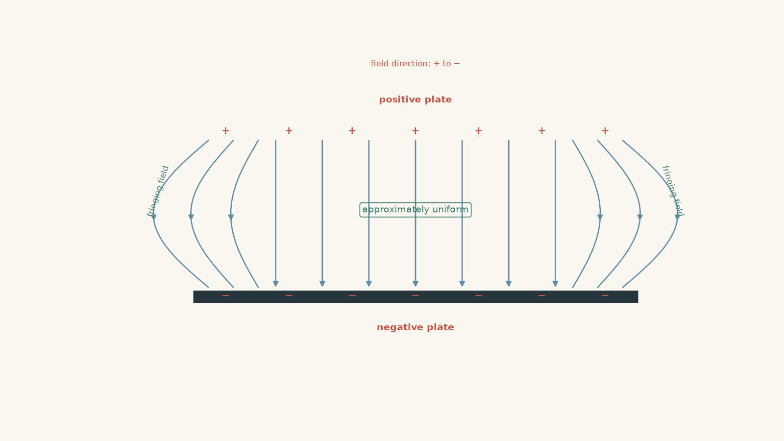
A useful mental picture is two enormous showerheads facing one another. In the middle, you could imagine the spray travelling in nearly straight, parallel paths. Near the rim, the spray can fan out.
The analogy has an important limit. Electric field lines are not streams of particles. They are a drawing tool that shows the direction and relative strength of the electric field.
02Why parallel plates produce an almost uniform field
Start with the idealised version.
Imagine the plates extend infinitely far in every sideways direction. There are no edges at all.
The electric field from the positive plate points away from it. The electric field from the negative plate points towards it.
Between the plates, those two fields point in the same direction, so they add.
Outside the plates, the two fields point in opposite directions and, for the ideal equal and opposite plates, cancel.
The result is an exactly uniform field between ideal infinite plates.
Real plates are finite, of course. Nobody has an infinitely wide aluminium plate tucked behind the physics lab.
However, if the plate width and height are much larger than the gap between them, a point near the centre does not “notice” the edges very much. The infinite-plate model becomes a good approximation there.
That gives us an important modelling rule:
Large plates, small separation, and a point well away from the edges means the uniform-field approximation is usually good.
There is no magical line where the field suddenly stops being uniform. The approximation gradually gets worse as you approach an edge.
03Field strength and potential difference
Suppose the plates have a potential difference \(\Delta V\) and are separated by a perpendicular distance \(d\).
Inside a uniform electric field, electric potential changes at a constant rate with distance. The magnitude of the field is therefore
\[
E = \frac{\Delta V}{d}
\]
where:
- \(E\) is the electric field strength, measured in volts per metre (\(\text{V m}^{-1}\)) or equivalently newtons per coulomb (\(\text{N C}^{-1}\))
- \(\Delta V\) is the magnitude of the potential difference between the plates, measured in volts (\(\text{V}\))
- \(d\) is the perpendicular separation of the plates, measured in metres (\(\text{m}\))
The direction of the electric field is from higher electric potential to lower electric potential, so it points from the positive plate towards the negative plate.
Notice what the equation is really saying. If the same voltage change happens over a smaller distance, the potential is changing more rapidly with position, so the electric field is stronger.
Worked example: Find the field and force between two plates
Two large parallel plates are separated by \(18\text{ mm}\) and maintained at a potential difference of \(450\text{ V}\). The left plate is positive. A particle with charge \(+3.0\text{ nC}\) is in the central region between the plates. Find the electric field strength and the electric force on the particle.
Step 1
\[
d = 18\text{ mm} = 0.018\text{ m}
\]
Step 2
\[
E = \frac{\Delta V}{d}
= \frac{450}{0.018}
= 2.5\times10^4\text{ V m}^{-1}
\]
The field points from the positive plate towards the negative plate, so here it points to the right.
Step 3
For a charge \(q\) in an electric field,
\[
F=qE
\]
where \(F\) is electric force in newtons and \(q\) is charge in coulombs.
The charge is
\[
q=+3.0\times10^{-9}\text{ C}
\]
so
\[
F=(3.0\times10^{-9})(2.5\times10^4)
=7.5\times10^{-5}\text{ N}
\]
Because the particle is positively charged, its force is in the same direction as the electric field.
The field is therefore \(2.5\times10^4\text{ V m}^{-1}\) to the right, and the particle experiences a force of \(7.5\times10^{-5}\text{ N}\) to the right.
The calculation assumes the particle is in the approximately uniform central region. Put it close enough to an edge, and \(E=\Delta V/d\) no longer tells you the exact local field.
04Why the field bends at the edges
Now return to real, finite plates.
Near the centre, charges on a plate are surrounded by lots of other plate surface in every sideways direction. The geometry is nearly symmetrical, which produces the familiar straight field through the gap.
Near an edge, that symmetry disappears. There is no conductor continuing beyond the edge to provide the same contribution to the field.
The electric field therefore bends around the ends of the plates. This is called an edge effect or fringing.
A fringing field has two important features:
- Its direction is no longer simply perpendicular to the broad faces of the plates.
- Its magnitude is not constant from point to point.
The field also extends outside the space directly between the plates. Real parallel plates therefore do not have a perfectly zero external field.
There is another layer of precision here. Charge on a real conducting plate is not necessarily spread with perfectly constant surface density. Charge tends to concentrate more strongly around edges and regions of greater curvature. Very close to an edge, the electric field can therefore be locally quite strong.
So avoid the oversimplification that “the electric field just gets weaker near the edge”. The safer statement is:
Near an edge, the field becomes nonuniform. Both its magnitude and direction can change.
05Why field lines meet a conductor at right angles
Look closely at a field diagram near one of the plates. Even when a field line is curving near an edge, it meets the conducting surface at right angles.
Why?
Suppose the electric field had a component along the surface of a conductor. Free electrons inside the conductor would feel a force along the surface and would move.
But in electrostatic equilibrium, the charges have already redistributed themselves so that there is no continuing motion of charge.
Therefore, the electric field at the surface cannot have a component parallel to the conductor. It must be perpendicular to the surface.
This also explains why the field direction can curve around the physical edge of a plate. “Perpendicular to the surface” changes direction as the geometry of the conductor changes.
06\(E=\Delta V/d\) is a model, not a magic formula
A common mistake is to see two parallel plates and immediately write
\[
E=\frac{\Delta V}{d}
\]
as though it gives the electric field at every point in space.
It does not.
The equation in this form assumes a uniform field. It works very well in the central region of large, closely spaced parallel plates.
Near an edge, the potential still changes through space, but not at the same constant rate in every direction. The field can have sideways and perpendicular components, so one value of \(\Delta V/d\) cannot describe the complete local field.
A useful decision table is:
| Situation | Useful model |
|---|---|
| Large plates, small gap, point near centre | Treat field as uniform and use \(E\approx\Delta V/d\) |
| Point approaching an edge | Expect fringing and changing field direction |
| Point outside finite plates | Do not assume \(E=0\) |
| Very close to a conductor edge | Expect strong local nonuniformity |
| Ideal infinite parallel plates | Field is exactly uniform between plates |
The word approximately is doing real work here.
07Potential also reveals whether the field is uniform
There is another way to recognise a uniform field.
Suppose you measure electric potential at equally spaced positions as you move directly from one plate to the other.
If the field is uniform, equal changes in distance produce equal changes in potential.
For example:
| Distance from negative plate | Potential |
|---|---|
| \(0\text{ mm}\) | \(0\text{ V}\) |
| \(5\text{ mm}\) | \(100\text{ V}\) |
| \(10\text{ mm}\) | \(200\text{ V}\) |
| \(15\text{ mm}\) | \(300\text{ V}\) |
| \(20\text{ mm}\) | \(400\text{ V}\) |
The potential increases by \(100\text{ V}\) every \(5\text{ mm}\). That constant rate of change corresponds to a constant field magnitude.
Near a plate edge, that neat relationship can break down because the electric field is no longer purely perpendicular to the plates or constant in magnitude.
This gives you two equivalent pictures of the central uniform region:
- field picture: straight, parallel, equally spaced field lines
- potential picture: potential changes linearly with perpendicular distance
08What happens to a charged particle in the uniform region?
Once the field is approximately uniform, the force on a particle is
\[
\vec F=q\vec E
\]
A positive charge accelerates in the direction of the field. A negative charge accelerates in the opposite direction.
Because \(E\) is constant in the uniform region, \(F\) is constant for a particle with fixed charge. Newton’s second law then gives
\[
a=\frac{F}{m}=\frac{qE}{m}
\]
where \(a\) is acceleration in \(\text{m s}^{-2}\) and \(m\) is the particle’s mass in kilograms.
That constant acceleration is why the uniform-field model is so useful.
Worked example: An electron moving between parallel plates
An electron enters horizontally through the central region between two parallel plates. The plates are \(20\text{ mm}\) apart and have a potential difference of \(30\text{ V}\). The upper plate is positive and the lower plate is negative. The plates are \(20\text{ mm}\) long in the direction of the electron’s motion.
The electron enters at \(6.0\times10^6\text{ m s}^{-1}\). Assuming a uniform field and ignoring fringing at the entrance and exit, calculate its vertical displacement while it is between the plates.
Use electron charge magnitude \(1.60\times10^{-19}\text{ C}\) and electron mass \(9.11\times10^{-31}\text{ kg}\).
Step 1
The plate separation is
\[
d=20\text{ mm}=0.020\text{ m}
\]
so
\[
E=\frac{\Delta V}{d}
=\frac{30}{0.020}
=1.5\times10^3\text{ V m}^{-1}
\]
The field points downwards, from the positive upper plate to the negative lower plate.
Step 2
An electron is negatively charged, so its force and acceleration are opposite the electric field. It therefore accelerates upwards.
The acceleration magnitude is
\[
a=\frac{|q|E}{m}
=\frac{(1.60\times10^{-19})(1.5\times10^3)}
{9.11\times10^{-31}}
=2.63\times10^{14}\text{ m s}^{-2}
\]
Step 3
There is no horizontal electric force in the ideal uniform-field model, so its horizontal velocity remains \(6.0\times10^6\text{ m s}^{-1}\).
The plate length is \(0.020\text{ m}\), giving
\[
t=\frac{x}{v_x}
=\frac{0.020}{6.0\times10^6}
=3.33\times10^{-9}\text{ s}
\]
Step 4
The electron initially has no vertical velocity, so
\[
\begin{aligned}
y&=\frac12at^2\\
&=\frac12(2.63\times10^{14})(3.33\times10^{-9})^2\\
&=1.46\times10^{-3}\text{ m}
\end{aligned}
\]
Therefore, the electron moves about
\[
\boxed{1.46\text{ mm}}
\]
upwards, towards the positive plate.
The physics is more important than the arithmetic: a uniform electric field produces a constant vertical force, so the vertical motion has constant acceleration while the horizontal motion continues at constant velocity.
The actual field at the entrance and exit would fringe rather than switching instantly on and off. The calculation deliberately ignores that small complication.
09The most tempting misconception: “parallel plates mean uniform field”
Not quite.
Infinite parallel plates with equal and opposite charge distributions give the ideal uniform field.
Finite parallel plates give an approximately uniform field only in a suitable central region.
That distinction becomes especially important when the plate separation is not small compared with the dimensions of the plates.
Imagine two square plates only \(20\text{ mm}\) wide but separated by \(15\text{ mm}\). There is barely any region that is comfortably far from an edge. Drawing perfectly straight field lines throughout the gap would be a poor model.
Now imagine plates \(500\text{ mm}\) wide separated by the same \(15\text{ mm}\). A point near their centre is much farther from an edge relative to the gap, so the uniform-field approximation is much better.
This is a general lesson in physics: an equation can be mathematically correct inside its model and still give a poor description if the model’s assumptions do not match the situation.
10Questions and solutions
Question 1
Two large parallel plates are \(25\text{ mm}\) apart and have a potential difference of \(750\text{ V}\). The upper plate is positive.
Calculate the electric field strength in the central region, including its direction.
Solution 1
The electric field is \(3.0\times10^4\text{ V m}^{-1}\) downwards, from the positive plate to the negative plate.
Convert the separation to metres:
\[
d=25\text{ mm}=0.025\text{ m}
\]
For the approximately uniform central field,
\[
E=\frac{\Delta V}{d}
=\frac{750}{0.025}
=3.0\times10^4\text{ V m}^{-1}
\]
Electric field direction is defined as the direction a positive test charge would accelerate. It therefore points from the positive upper plate towards the negative lower plate.
The important assumption is that the point considered is in the central region where edge effects are negligible.
Question 2
An electron is placed at rest in a uniform electric field of magnitude \(1.2\times10^4\text{ N C}^{-1}\) directed to the left.
Calculate the initial electric force on the electron, and state its direction.
Use an electron charge of \(-1.60\times10^{-19}\text{ C}\).
Solution 2
The electron experiences a force of \(1.92\times10^{-15}\text{ N}\) to the right.
The magnitude of electric force is
\[
F=|q|E
\]
so
\[
\begin{aligned}
F&=(1.60\times10^{-19})(1.2\times10^4)\\
&=1.92\times10^{-15}\text{ N}
\end{aligned}
\]
The field points to the left, but an electron has negative charge. Its electric force is therefore opposite the field, so the force points to the right.
A common mistake is to calculate the correct magnitude and then send the electron in the field direction. Positive charges accelerate with the field. Negative charges accelerate against it.
Question 3
A pair of rectangular parallel plates is connected to a constant \(600\text{ V}\) supply. Their separation is increased from \(10\text{ mm}\) to \(20\text{ mm}\), while their width and height remain unchanged.
Describe two changes you would expect:
- the approximate electric field strength near the centre
- the importance of edge effects
Solution 3
The central field strength approximately halves, while edge effects become more significant relative to the central uniform region.
Initially,
\[
E_1=\frac{600}{0.010}
=6.0\times10^4\text{ V m}^{-1}
\]
After the separation is doubled,
\[
E_2=\frac{600}{0.020}
=3.0\times10^4\text{ V m}^{-1}
\]
So the approximate central field strength halves.
The second change cannot be found from \(E=\Delta V/d\) alone. Increasing the separation while leaving the plate dimensions unchanged makes the gap larger compared with the width and height of the plates. The edges therefore have more influence over the region between the plates.
The tempting mistake is to discuss only the numerical field strength. The geometry also determines how good the uniform-field model is.
Question 4
Two students investigate plates separated by \(12\text{ mm}\) with a potential difference of \(300\text{ V}\).
Student A calculates
\[
E=\frac{300}{0.012}=2.5\times10^4\text{ V m}^{-1}
\]
Student B uses a field probe at several points. Near the centre, the probe reads close to \(2.5\times10^4\text{ V m}^{-1}\), but near one edge the readings vary in both magnitude and direction.
Student A says the probe must be faulty because \(E=\Delta V/d\) gives only one value.
Evaluate Student A’s conclusion.
Solution 4
Student A’s conclusion is incorrect. The measurements are consistent with edge effects from finite parallel plates.
The calculation
\[
E=\frac{\Delta V}{d}
=\frac{300}{0.012}
=2.5\times10^4\text{ V m}^{-1}
\]
is appropriate for the approximately uniform central region.
It does not prove that every point between real finite plates has exactly that field.
Near an edge, field lines fringe outwards. The electric field can therefore change in both magnitude and direction. The probe reading near the centre agreeing with \(2.5\times10^4\text{ V m}^{-1}\) actually supports the uniform-field approximation where it should work.
Student A has treated a model assumption as an exact property of the real apparatus. That is the trap.
Question 5
A positively charged oil droplet has mass \(2.0\times10^{-12}\text{ kg}\) and charge \(+4.0\times10^{-15}\text{ C}\). It is initially held stationary halfway between two horizontal parallel plates separated by \(8.0\text{ mm}\).
Assume the droplet begins in the uniform central region.
Calculate the potential difference required to balance its weight. Then explain why the same potential difference may fail to keep the droplet stationary if it drifts sideways towards an edge of the plates.
Use \(g=9.8\text{ m s}^{-2}\).
Solution 5
A potential difference of approximately \(39\text{ V}\) is required in the central uniform region, but the droplet may no longer remain stationary near an edge because the local electric field changes in magnitude and direction.
For the droplet to remain stationary, the upward electric force must equal its downward weight:
\[
qE=mg
\]
Therefore,
\[
E=\frac{mg}{q}
\]
Substituting,
\[
\begin{aligned}
E&=\frac{(2.0\times10^{-12})(9.8)}
{4.0\times10^{-15}}\\
&=4.9\times10^3\text{ N C}^{-1}
\end{aligned}
\]
For a uniform field,
\[
E=\frac{\Delta V}{d}
\]
so
\[
\begin{aligned}
\Delta V&=Ed\\
&=(4.9\times10^3)(8.0\times10^{-3})\\
&=39.2\text{ V}
\end{aligned}
\]
Thus the required potential difference is approximately
\[
\boxed{39\text{ V}}
\]
For the electric force to point upwards on a positive droplet, the electric field must point upwards. The lower plate must therefore be positive relative to the upper plate.
Near an edge, however, the field is no longer the same vertical vector used in the calculation. Fringing gives the field a sideways component, and its vertical component can differ from the central value.
That means the condition \(qE=mg\), with the electric force exactly upwards, may no longer hold. The droplet can accelerate vertically, sideways, or both.
The hidden assumption was not the force equation. \(F=qE\) still applies. The hidden assumption was that the same uniform electric field exists everywhere between the plates.
11What this lets you do next
Once you can decide where the parallel-plate field is reasonably uniform, charged-particle motion becomes much easier to model. In the central region, \(F=qE\) is constant, so the particle has constant acceleration in the field direction.
That leads directly to electron beams, charged-particle deflection, and situations where electric and magnetic forces act together. The important habit carries with you: before using the neat equation, identify the physical assumptions that make it neat.