
Maxwell’s Prediction of the Speed of Light: HSC Physics
Learn how Maxwell connected the electromagnetic constants to a predicted wave speed and why its match with the speed of light was so important. Includes worked examples and challenging HSC-style questions.
Imagine you had never measured the speed of light. You only knew how strongly electric charges push on each other, and how strongly electric currents produce magnetic fields. Could those measurements tell you how fast light travels?
Maxwell’s equations say yes. They contain two electromagnetic constants, \(\varepsilon_0\) and \(\mu_0\), and when those constants are combined, a speed falls out:
\[ v=\frac{1}{\sqrt{\mu_0\varepsilon_0}} \]
Before calculating it, make a prediction. If that speed happened to match the measured speed of light, would you treat that as a random coincidence?
Maxwell didn’t. The match was the clue that light itself is an electromagnetic wave.
01A speed hiding inside electricity and magnetism
The two constants look fairly harmless when you first meet them.
| Constant | Name | What it helps set | Approximate value |
|---|---|---|---|
| \(\varepsilon_0\) | permittivity of free space | strength of electric-field effects in vacuum | \(8.85\times10^{-12}\ \mathrm{F\,m^{-1}}\) |
| \(\mu_0\) | permeability of free space | strength of magnetic-field effects in vacuum | \(1.26\times10^{-6}\ \mathrm{H\,m^{-1}}\) |
You can see \(\varepsilon_0\) in Coulomb’s law:
\[ F=\frac{1}{4\pi\varepsilon_0}\frac{q_1q_2}{r^2} \]
Here, \(F\) is the electric force in newtons, \(q_1\) and \(q_2\) are charges in coulombs, and \(r\) is their separation in metres.
You can see \(\mu_0\) in the magnetic field around a long straight current-carrying wire:
\[ B=\frac{\mu_0 I}{2\pi r} \]
Here, \(B\) is magnetic field strength in tesla, \(I\) is current in amperes, and \(r\) is distance from the wire in metres.
At first, these equations seem to describe static situations: charges sitting there, or a steady current flowing through a wire. Nothing here obviously screams “light”.
That changes when the fields vary with time.
02How Maxwell turns fields into a wave
Faraday’s law connects a changing magnetic field to an electric field. The Ampère-Maxwell law connects a changing electric field to a magnetic field.
So imagine a disturbance in an electric field. The equations don’t let that disturbance remain purely electric. Electric and magnetic behaviour are coupled, allowing the disturbance to propagate through space.
A useful comparison is a wave on a stretched string. The speed of the string wave isn’t chosen by the person shaking the string. It depends on properties of the system, such as the tension and the mass per unit length.
Electromagnetic waves have the same broad idea: their propagation speed is set by quantities already present in the governing equations.
The analogy stops there. Empty space is not literally a material string, and \(\varepsilon_0\) and \(\mu_0\) are not evidence for some hidden substance that light needs to travel through.
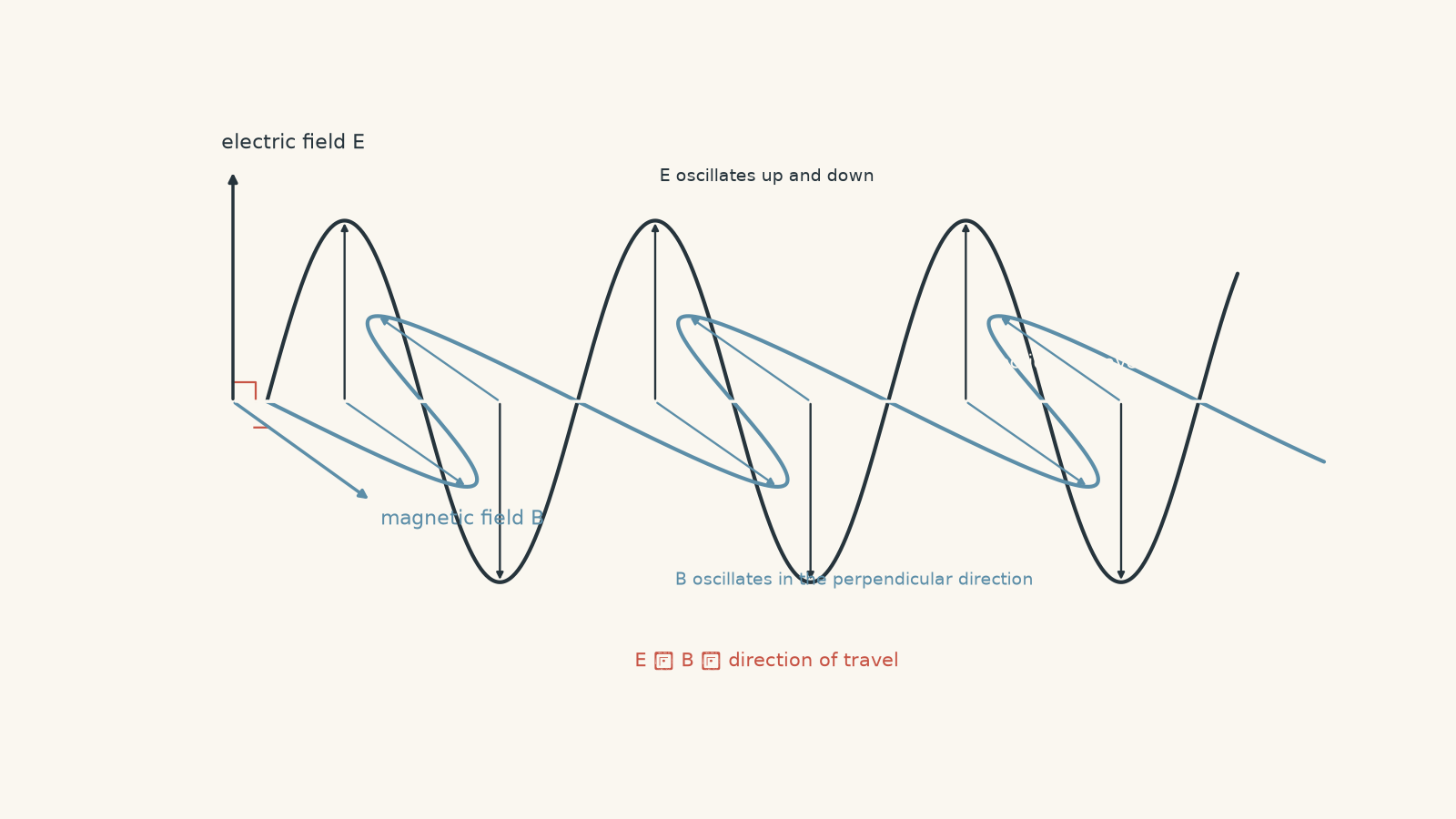
When Maxwell’s equations are combined in empty space, they produce a wave equation. For one component of the electric field, its structure is
\[ \frac{\partial^2 E}{\partial x^2} = \mu_0\varepsilon_0 \frac{\partial^2 E}{\partial t^2} \]
Here, \(E\) is the electric-field component, \(x\) is position, and \(t\) is time.
You do not need to get distracted by the derivative notation to see the important move. A general one-dimensional wave equation has the form
\[ \frac{\partial^2 y}{\partial x^2} = \frac{1}{v^2} \frac{\partial^2 y}{\partial t^2} \]
where \(y\) is whatever quantity is waving, and \(v\) is the wave speed.
Compare the coefficients:
\[ \frac{1}{v^2}=\mu_0\varepsilon_0 \]
Therefore,
\[ v^2=\frac{1}{\mu_0\varepsilon_0} \]
and hence
\[ v=\frac{1}{\sqrt{\mu_0\varepsilon_0}} \]
That is Maxwell’s prediction.
Notice what has happened. We have not inserted the measured speed of light anywhere. The speed comes from the equations of electricity and magnetism.
Worked example: Recover the speed of light
Use \(\mu_0=1.26\times10^{-6}\ \mathrm{H\,m^{-1}}\) and \(\varepsilon_0=8.85\times10^{-12}\ \mathrm{F\,m^{-1}}\) to calculate the electromagnetic wave speed predicted by Maxwell’s equations.
Step 1
\[ v=\frac{1}{\sqrt{\mu_0\varepsilon_0}} \]
Step 2
\[ v= \frac{1}{ \sqrt{ (1.26\times10^{-6}) (8.85\times10^{-12}) } } \]
Step 3
\[ \mu_0\varepsilon_0 = 1.115\times10^{-17}\ \mathrm{s^2\,m^{-2}} \]
The units are worth checking. Since \(\mathrm{H\,F}=\mathrm{s^2}\),
\[ (\mathrm{H\,m^{-1}})(\mathrm{F\,m^{-1}}) = \mathrm{s^2\,m^{-2}} \]
Taking the square root gives \(\mathrm{s\,m^{-1}}\), and taking the reciprocal gives \(\mathrm{m\,s^{-1}}\), exactly the unit a speed should have.
Step 4
\[ v = \frac{1}{\sqrt{1.115\times10^{-17}}} \approx 2.99\times10^8\ \mathrm{m\,s^{-1}} \]
So Maxwell’s electromagnetic equations predict a wave speed of about
\[ v\approx3.00\times10^8\ \mathrm{m\,s^{-1}} \]
That is the speed of light in vacuum to the precision of the rounded constants used here.
03Why that numerical match mattered
In the nineteenth century, the speed of light had already been estimated using optical measurements. Maxwell approached the problem from a completely different direction: electricity and magnetism.
His theory produced electromagnetic waves with a predicted speed close to the independently measured speed of light.
That is much stronger than simply noticing that two things move quickly. The equations predicted a particular speed before “light” had to be inserted into the calculation. Maxwell argued that light was therefore an electromagnetic disturbance.
This speed result is one part of the larger argument developed in Maxwell’s Prediction of Electromagnetic Waves.
It is still worth being careful with the logic. A matching speed is strong evidence for the identification, but a numerical match by itself is not a magical proof. The full theory also makes predictions about the electric and magnetic structure, propagation, and behaviour of electromagnetic waves.
04What happens if the constants change?
From
\[ v=\frac{1}{\sqrt{\mu\varepsilon}} \]
you can see that wave speed depends on the product \(\mu\varepsilon\).
This leads to a useful decision rule:
- if \(\mu\varepsilon\) increases, \(v\) decreases;
- if \(\mu\varepsilon\) decreases, \(v\) increases;
- if \(\mu\varepsilon\) stays unchanged, \(v\) stays unchanged.
The square root matters. Doubling the product does not halve the speed. It changes the speed by a factor of \(1/\sqrt{2}\).
For comparisons with vacuum, it is often cleaner to divide the two speed equations:
\[ \frac{v}{c} = \sqrt{ \frac{\mu_0\varepsilon_0}{\mu\varepsilon} } \]
Here, \(c\) is the electromagnetic wave speed in vacuum.
Worked example: Change both constants
A hypothetical region has permittivity \(\varepsilon=1.44\varepsilon_0\) and permeability \(\mu=0.81\mu_0\). Assuming the simple electromagnetic-wave model applies, find the wave speed.
Step 1
\[ \frac{v}{c} = \sqrt{ \frac{\mu_0\varepsilon_0} {(0.81\mu_0)(1.44\varepsilon_0)} } \]
Step 2
\[ \frac{v}{c} = \frac{1}{\sqrt{0.81\times1.44}} \]
Step 3
\[ 0.81\times1.44=1.1664 \]
so
\[ \frac{v}{c} = \frac{1}{\sqrt{1.1664}} = \frac{1}{1.08} = 0.926 \]
Step 4
Using \(c=3.00\times10^8\ \mathrm{m\,s^{-1}}\),
\[ v = 0.926(3.00\times10^8) = 2.78\times10^8\ \mathrm{m\,s^{-1}} \]
The wave is about \(7.4\%\) slower than light in vacuum.
The tempting prediction is that the lower \(\mu\) should make the wave faster, so perhaps the two changes simply cancel. They do not. What matters is their product, and here
\[ (0.81)(1.44)=1.1664 \]
so \(\mu\varepsilon\) has increased overall.
05The constants are not electromagnetic “drag”
A common mental picture is that a large permittivity or permeability makes space somehow “thicker”, so the wave has to fight its way through.
That picture becomes misleading quickly.
Neither \(\varepsilon_0\) nor \(\mu_0\) is a friction coefficient. A vacuum electromagnetic wave does not steadily lose energy simply because those constants are non-zero. The constants set relationships between electric and magnetic quantities in Maxwell’s equations, and their product determines the wave speed.
There is another tempting oversimplification: “The electric field creates the magnetic field, then the magnetic field creates another electric field, and they take turns forever.”
That is useful for about ten seconds.
More precisely, the spatial and time variations of the electric and magnetic fields are coupled by Maxwell’s equations. In a travelling sinusoidal electromagnetic wave in vacuum, the electric and magnetic fields oscillate together rather than politely taking turns like two people sending increasingly desperate texts.
06Vacuum first, materials second
In vacuum,
\[ c=\frac{1}{\sqrt{\mu_0\varepsilon_0}} \]
For a simple homogeneous, linear material, the corresponding model is
\[ v=\frac{1}{\sqrt{\mu\varepsilon}} \]
where \(\mu\) and \(\varepsilon\) describe the material.
Real materials can be more complicated. Their electromagnetic response may depend on frequency, and they can absorb energy. For HSC-style calculations using this relationship, assume the quoted \(\mu\) and \(\varepsilon\) are suitable effective values unless the question says otherwise.
Once the wave speed is known, the usual wave equation still applies:
\[ v=f\lambda \]
where \(f\) is frequency in hertz and \(\lambda\) is wavelength in metres.
When a wave crosses from one medium into another, its frequency is fixed by the source and remains continuous across the boundary. If the speed changes, the wavelength changes with it.
That distinction becomes important when you connect Maxwell’s result to the electromagnetic spectrum.
07One modern wrinkle: today’s SI changes what counts as an independent test
There is a subtle difference between Maxwell’s historical calculation and plugging modern tabulated constants into a calculator.
In the modern SI, the speed of light in vacuum is assigned the exact value
\[ c=299\,792\,458\ \mathrm{m\,s^{-1}} \]
and has been used in the definition of the metre since 1983. Since the 2019 revision of the SI, \(\mu_0\) is no longer assigned its old exact numerical value. However, the electromagnetic constants still obey the exact relation
\[ \mu_0\varepsilon_0=\frac{1}{c^2} \]
within SI. BIPM
So if you take modern, self-consistent tabulated SI values of \(\mu_0\) and \(\varepsilon_0\), substitute them into Maxwell’s formula, and recover \(c\), you have checked that the numbers are mutually consistent. You have not recreated the same independent historical comparison Maxwell made between electromagnetic measurements and optical measurements.
This is closely connected to why the speed of light now defines the metre.
08Questions and solutions
Question 1
In a hypothetical region, the product of permeability and permittivity is
\[ \mu\varepsilon=1.60\times10^{-17}\ \mathrm{s^2\,m^{-2}} \]
Calculate:
a. the electromagnetic wave speed in the region;
b. the time required for the wave to travel \(750\ \mathrm{m}\).
Solution 1
The wave speed is \(2.50\times10^8\ \mathrm{m\,s^{-1}}\), and the \(750\ \mathrm{m}\) journey takes \(3.00\times10^{-6}\ \mathrm{s}\).
For part a, Maxwell’s wave-speed relationship gives
\[ v=\frac{1}{\sqrt{\mu\varepsilon}} \]
Substituting,
\[ v = \frac{1}{ \sqrt{1.60\times10^{-17}} } \]
Since
\[ \sqrt{1.60\times10^{-17}} = 4.00\times10^{-9}\ \mathrm{s\,m^{-1}} \]
we obtain
\[ v = \frac{1}{4.00\times10^{-9}} = 2.50\times10^8\ \mathrm{m\,s^{-1}} \]
For part b,
\[ t=\frac{d}{v} \]
so
\[ t = \frac{750} {2.50\times10^8} = 3.00\times10^{-6}\ \mathrm{s} \]
The main trap is forgetting the square root and calculating \(1/(\mu\varepsilon)\). That would not even have the units of speed.
Question 2
An electromagnetic wave travels through a hypothetical vacuum-like region at \(2.80\times10^8\ \mathrm{m\,s^{-1}}\). The permeability of the region is \(1.20\times10^{-6}\ \mathrm{H\,m^{-1}}\).
a. Calculate its permittivity.
b. Compare your value with \(\varepsilon_0=8.85\times10^{-12}\ \mathrm{F\,m^{-1}}\).
c. Explain why knowing only that the wave travels more slowly than light in vacuum does not tell you whether the change occurred in permeability, permittivity, or both.
Solution 2
The permittivity is \(1.06\times10^{-11}\ \mathrm{F\,m^{-1}}\), about \(20\%\) greater than \(\varepsilon_0\); the wave speed alone cannot tell us which individual constant changed because it constrains only their product.
Starting with
\[ v=\frac{1}{\sqrt{\mu\varepsilon}} \]
square both sides:
\[ v^2=\frac{1}{\mu\varepsilon} \]
Rearrange for \(\varepsilon\):
\[ \varepsilon=\frac{1}{\mu v^2} \]
Substitute the values:
\[ \begin{aligned} \varepsilon &= \frac{1}{ (1.20\times10^{-6}) (2.80\times10^8)^2 }\\ &= \frac{1}{ (1.20\times10^{-6})(7.84\times10^{16}) }\\ &= 1.06\times10^{-11}\ \mathrm{F\,m^{-1}} \end{aligned} \]
Compare this with \(\varepsilon_0\):
\[ \frac{\varepsilon}{\varepsilon_0} = \frac{1.06\times10^{-11}} {8.85\times10^{-12}} \approx1.20 \]
so the permittivity is about \(20\%\) larger.
For part c, the governing constraint is
\[ \mu\varepsilon=\frac{1}{v^2} \]
A measurement of \(v\) therefore determines the product \(\mu\varepsilon\), not \(\mu\) and \(\varepsilon\) separately. Many different pairs could produce the same wave speed.
The tempting route is to blame the slower speed on the given permeability. But without an independent measurement of at least one constant, speed alone cannot separate their effects.
Question 3
A monochromatic electromagnetic wave of frequency \(2.00\times10^8\ \mathrm{Hz}\) travels through a homogeneous material with wavelength \(1.20\ \mathrm{m}\). Assume \(\mu=\mu_0\), and take \(c=3.00\times10^8\ \mathrm{m\,s^{-1}}\).
a. Calculate the wave speed in the material.
b. Find \(\varepsilon/\varepsilon_0\).
c. The wave then leaves the material and enters vacuum. State its frequency and wavelength in vacuum, and explain which quantity changes at the boundary.
Solution 3
The wave travels at \(2.40\times10^8\ \mathrm{m\,s^{-1}}\), the material has \(\varepsilon=1.56\varepsilon_0\), and on entering vacuum the frequency remains \(2.00\times10^8\ \mathrm{Hz}\) while the wavelength increases to \(1.50\ \mathrm{m}\).
For part a, use
\[ v=f\lambda \]
so
\[ v = (2.00\times10^8)(1.20) = 2.40\times10^8\ \mathrm{m\,s^{-1}} \]
For part b,
\[ v=\frac{1}{\sqrt{\mu_0\varepsilon}} \]
while in vacuum,
\[ c=\frac{1}{\sqrt{\mu_0\varepsilon_0}} \]
Divide the equations:
\[ \frac{c}{v} = \sqrt{\frac{\varepsilon}{\varepsilon_0}} \]
because \(\mu=\mu_0\).
Squaring gives
\[ \frac{\varepsilon}{\varepsilon_0} = \left(\frac{c}{v}\right)^2 \]
Therefore,
\[ \frac{\varepsilon}{\varepsilon_0} = \left( \frac{3.00\times10^8} {2.40\times10^8} \right)^2 = (1.25)^2 = 1.5625 \]
so
\[ \varepsilon\approx1.56\varepsilon_0 \]
For part c, the frequency remains
\[ f=2.00\times10^8\ \mathrm{Hz} \]
because the oscillation rate is set by the source. Once the wave returns to vacuum, its speed becomes \(c\), so
\[ \lambda_0=\frac{c}{f} \]
and
\[ \lambda_0 = \frac{3.00\times10^8} {2.00\times10^8} = 1.50\ \mathrm{m} \]
The tempting prediction is that a slower wave must oscillate more slowly. Instead, at an ordinary stationary boundary, the frequency stays fixed and the wavelength adjusts to the new speed.
Question 4
A hypothetical homogeneous region \(X\) behaves according to the usual electromagnetic equations.
Experiments reveal two facts:
- two fixed charges separated by the same distance experience only \(\frac{2}{3}\) of the force they would experience in vacuum;
- electromagnetic waves in region \(X\) travel at exactly the vacuum speed \(c\).
Determine:
a. \(\varepsilon_X/\varepsilon_0\);
b. \(\mu_X/\mu_0\);
c. the ratio \(B_X/B_0\) for the magnetic field at the same distance from the same long straight wire carrying the same current.
A student argues that because the wave speed is unchanged, both electromagnetic constants must have their vacuum values. Explain exactly where that reasoning fails.
Solution 4
The required ratios are \(\varepsilon_X/\varepsilon_0=3/2\), \(\mu_X/\mu_0=2/3\), and \(B_X/B_0=2/3\); an unchanged wave speed fixes the product \(\mu\varepsilon\), not the two constants individually.
First use Coulomb’s law. For fixed charges and separation,
\[ F\propto\frac{1}{\varepsilon} \]
Therefore,
\[ \frac{F_X}{F_0} = \frac{\varepsilon_0}{\varepsilon_X} \]
The question gives
\[ \frac{F_X}{F_0}=\frac{2}{3} \]
so
\[ \frac{2}{3} = \frac{\varepsilon_0}{\varepsilon_X} \]
and hence
\[ \varepsilon_X=\frac{3}{2}\varepsilon_0 \]
For part b, the wave speed is unchanged:
\[ \frac{1}{\sqrt{\mu_X\varepsilon_X}} = \frac{1}{\sqrt{\mu_0\varepsilon_0}} \]
Therefore,
\[ \mu_X\varepsilon_X = \mu_0\varepsilon_0 \]
Substitute \(\varepsilon_X=\frac{3}{2}\varepsilon_0\):
\[ \mu_X \left(\frac{3}{2}\varepsilon_0\right) = \mu_0\varepsilon_0 \]
so
\[ \mu_X=\frac{2}{3}\mu_0 \]
For part c, the field around a long straight wire is
\[ B=\frac{\mu I}{2\pi r} \]
With \(I\) and \(r\) unchanged,
\[ B\propto\mu \]
so
\[ \frac{B_X}{B_0} = \frac{\mu_X}{\mu_0} = \frac{2}{3} \]
The student’s mistake is subtle. Starting from
\[ v=\frac{1}{\sqrt{\mu\varepsilon}} \]
the condition \(v_X=c\) tells us
\[ \mu_X\varepsilon_X=\mu_0\varepsilon_0 \]
It does not require
\[ \mu_X=\mu_0 \]
and
\[ \varepsilon_X=\varepsilon_0 \]
separately.
Here, one constant increases by a factor of \(3/2\) while the other decreases by a factor of \(2/3\). Their product is unchanged, so the wave speed remains unchanged even though the static electric and magnetic responses are both different from vacuum.
That is why measuring wave speed alone cannot reconstruct both electromagnetic constants.
Question 5
In 2026, a student looks up tabulated SI values of \(\mu_0\) and \(\varepsilon_0\), calculates
\[ \frac{1}{\sqrt{\mu_0\varepsilon_0}} \]
and obtains \(299\,792\,458\ \mathrm{m\,s^{-1}}\).
They conclude:
“I have independently verified Maxwell’s nineteenth-century prediction in exactly the same way Maxwell did.”
Assess this conclusion. Your answer should distinguish between:
- Maxwell’s physical prediction;
- the historical comparison with measured light speed; and
- the status of \(c\), \(\mu_0\), and \(\varepsilon_0\) in the modern SI.
Solution 5
The student’s calculation is consistent with Maxwell’s electromagnetic relationship, but it is not an independent modern experimental verification of the same kind as Maxwell’s historical comparison.
Maxwell’s physical prediction comes from the structure of his electromagnetic equations. They imply that disturbances in the electric and magnetic fields can propagate with speed
\[ v=\frac{1}{\sqrt{\mu_0\varepsilon_0}} \]
The remarkable historical step was then to compare a speed obtained from electromagnetic quantities with a speed obtained independently from optical measurements. Their close agreement supported Maxwell’s identification of light as an electromagnetic wave.
The modern calculation has a different logical structure.
In today’s SI, the speed of light in vacuum is assigned the exact numerical value
\[ c=299\,792\,458\ \mathrm{m\,s^{-1}} \]
and the electromagnetic constants obey
\[ \varepsilon_0\mu_0=\frac{1}{c^2} \]
exactly. Since the 2019 SI revision, \(\mu_0\) itself is no longer assigned the old exact value \(4\pi\times10^{-7}\ \mathrm{H\,m^{-1}}\), but \(\varepsilon_0\), \(\mu_0\), and \(c\) are not three freely independent tabulated numbers. BIPM
Therefore,
\[ \frac{1}{\sqrt{\mu_0\varepsilon_0}} = \frac{1}{\sqrt{1/c^2}} = c \]
must follow for a self-consistent set of SI values.
The tempting route is to see an impressive numerical agreement and assume that two independent measurements have met in the middle. In the modern calculation, that independence is the missing constraint. The constants have already been related within the SI framework.
This does not weaken Maxwell’s historical achievement, nor does it mean electromagnetic theory cannot be experimentally tested. It means only that this particular plug-in calculation, using modern SI tabulated constants, is not a fresh independent test.
09What this result unlocks next
Maxwell’s important move was not simply calculating a very large number. It was discovering that the equations governing electric and magnetic fields contain their own wave speed, and that this speed matched light.
Once light is recognised as electromagnetic radiation, the familiar wave relationship
\[ c=f\lambda \]
connects every vacuum electromagnetic wave to its frequency and wavelength. Radio waves, microwaves, infrared, visible light, ultraviolet, X-rays, and gamma rays differ enormously in \(f\) and \(\lambda\), but Maxwell’s theory puts them in the same electromagnetic family.
That is the bridge from Maxwell’s equations to the electromagnetic spectrum, and from there to ideas such as continuous, emission, and absorption spectra.