
Millikan’s Oil-Drop Experiment: HSC Physics Explained
Understand how Millikan measured the elementary charge, showed that charge is quantised, and combined his result with Thomson's work to determine electron mass.
By the early 1900s, physicists had strong evidence that atoms contained tiny negatively charged particles. J. J. Thomson’s cathode-ray experiments had even measured the electron’s charge-to-mass ratio, \(e/m\). But there was a stubborn problem: knowing a ratio is not the same as knowing either quantity separately.
Imagine being told that two people’s heights are in the ratio \(2:1\). You still don’t know whether they are 2 m and 1 m tall, or 1.6 m and 0.8 m tall. Thomson faced the same problem. To find the electron’s mass, physicists needed an independent measurement of its charge.
Robert Millikan’s oil-drop experiment supplied that missing measurement. More importantly, the experiment showed that electric charge comes in discrete units: the charges on the drops were always whole-number multiples of one smallest value.
That smallest value is the elementary charge,
\[ e \approx 1.60\times10^{-19}\ \text{C}. \]
Once \(e\) was combined with Thomson’s earlier measurement of \(e/m\), the electron’s mass could be calculated.
01What exactly had to be measured?
Suppose a tiny object has somehow picked up extra electrons. Its charge might be
\[ -e,\quad -2e,\quad -3e,\quad \ldots \]
but in Millikan’s time that pattern was something to test, not something to assume.
The experimental problem was nasty. An electron is far too small to place on a balance. Its mass is about \(9.11\times10^{-31}\) kg. Even a speck of dust contains an enormous number of atoms.
So Millikan’s strategy was indirect: put a small electric charge onto an object large enough to observe, then use forces to work backwards to the charge.
The object was a microscopic oil drop.
Why oil? Because a tiny oil droplet can remain stable long enough to watch. A water droplet gradually evaporates, changing its radius and therefore its mass while you are trying to measure it. That is exactly the sort of experimental annoyance that can quietly ruin an otherwise clever method.
02Picture the apparatus
The central part of the experiment contained two horizontal metal plates, one above the other, separated by a small distance.
A voltage was applied across the plates, creating an approximately uniform electric field between them.
Above the upper plate was an atomiser. It sprayed extremely small oil droplets into the apparatus. Some droplets passed through a tiny hole in the upper plate and entered the gap between the plates.
The drops acquired electric charge, commonly through ionisation processes that transferred electrons to or from them.
A lamp illuminated the droplets from the side. Millikan observed individual droplets through a microscope.
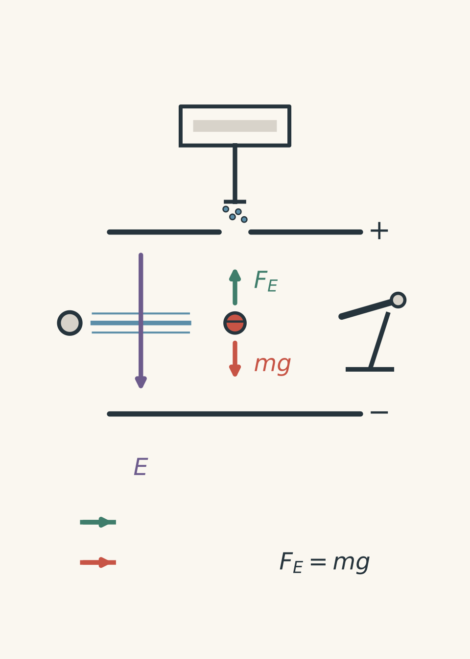
Mentally follow one drop.
It leaves the atomiser, passes through the hole, enters the space between the plates, and falls under gravity. Millikan observes its motion through the microscope.
Then the electric field is switched on.
If the field has the correct direction and strength, the electric force can oppose gravity. Adjust the voltage carefully enough, and the droplet can be held almost motionless.
That stationary drop is the key measurement.
03Predict the force balance
Suppose a negatively charged drop is hanging motionless between the plates.
What must be true about the forces?
A common first thought is that gravity has somehow stopped acting. It hasn’t. The drop is stationary because the forces balance.
Gravity pulls downward. The electric force pulls upward.
In the simplest HSC model,
\[ F_g=mg \]
and
\[ F_E=qE, \]
where:
- \(m\) is the mass of the oil drop in kilograms,
- \(g\) is gravitational field strength in \(\text{m s}^{-2}\),
- \(q\) is the magnitude of the drop’s charge in coulombs, and
- \(E\) is the electric field strength in \(\text{N C}^{-1}\).
For a stationary drop,
\[ F_E=F_g, \]
so
\[ qE=mg. \]
Therefore,
\[ q=\frac{mg}{E}. \]
If the plates are approximately parallel and edge effects can be neglected,
\[ E=\frac{V}{d}, \]
where \(V\) is the potential difference between the plates and \(d\) is their separation.
Combining the equations gives
\[ q=\frac{mgd}{V}. \]
This is the neat part. If you know the drop’s mass, plate separation, and balancing voltage, you can calculate its charge.
But there is an obvious problem hiding inside that sentence.
How do you know the mass of something microscopic?
04The falling drop reveals its size
Millikan could not simply take one droplet out and put it on a laboratory balance.
Instead, its motion through air gave information about its size.
When a tiny sphere falls through air, gravity initially makes it accelerate. As its speed increases, air resistance increases. Eventually the upward resistive force becomes large enough that the net force approaches zero.
The droplet then falls at a constant speed called its terminal velocity.
For a sufficiently small sphere moving slowly through a fluid, Stokes’ law gives the drag force as
\[ F_D=6\pi\eta rv, \]
where:
- \(\eta\) is the dynamic viscosity of air,
- \(r\) is the radius of the droplet, and
- \(v\) is its speed.
At terminal velocity, the downward gravitational effect is balanced by upward drag and buoyancy.
A simple classroom treatment may write
\[ mg=6\pi\eta rv. \]
A more accurate treatment includes the buoyant force from displaced air. Then the effective downward force is
\[ F_{\text{effective}}= \frac{4}{3}\pi r^3(\rho_{\text{oil}}-\rho_{\text{air}})g. \]
At terminal speed \(v_t\),
\[ 6\pi\eta rv_t= \frac{4}{3}\pi r^3(\rho_{\text{oil}}-\rho_{\text{air}})g. \]
Solving for \(r\),
\[ r= \sqrt{ \frac{9\eta v_t} {2(\rho_{\text{oil}}-\rho_{\text{air}})g} }. \]
Once the radius is known, the oil drop’s volume is
\[ V_{\text{drop}}=\frac{4}{3}\pi r^3, \]
and its mass is approximately
\[ m=\rho_{\text{oil}}V_{\text{drop}}. \]
So the experiment links two observations:
- how quickly the drop falls when gravity and air resistance control its motion, and
- what electric field is required to balance it.
From those measurements, its charge can be inferred.
The first mental model, \(qE=mg\), is useful. It captures the main idea. But the actual measurement requires greater care because air resistance, buoyancy, droplet size, viscosity, and very small-scale corrections affect the result.
05Why use oil instead of water?
An earlier difficulty with experiments involving tiny droplets was that the droplets could evaporate.
Imagine trying to measure someone’s mass while they are steadily disappearing. A little inconvenient.
If a water droplet shrinks, its radius changes. Its volume changes as \(r^3\), so its mass changes too. Its terminal speed also changes. That makes it much harder to know whether a change in motion came from electric charge or simply from evaporation.
Using a much less volatile oil made individual droplets more stable over the measurement period.
This did not make the experiment perfect. Millikan still had to account for the behaviour of tiny spheres moving through air, and refinements were required to Stokes’ law at very small scales. But the oil-drop design greatly improved the ability to follow the same droplet for long enough to make repeated measurements.
06Worked example: finding the charge on a suspended drop
An oil droplet of mass \(4.8\times10^{-15}\) kg is stationary between two horizontal parallel plates. The electric field strength is \(9.8\times10^4\ \text{N C}^{-1}\). Calculate the magnitude of the charge on the drop.
Take \(g=9.8\ \text{m s}^{-2}\).
Step 1
Its acceleration is zero, so the net force is zero. In the simplified model,
\[ qE=mg. \]
Step 2
\[ q=\frac{mg}{E}. \]
Step 3
\[ q= \frac{(4.8\times10^{-15}\ \text{kg})(9.8\ \text{m s}^{-2})} {9.8\times10^4\ \text{N C}^{-1}}. \]
Since \(1\ \text{N}=1\ \text{kg m s}^{-2}\),
\[ q=4.8\times10^{-19}\ \text{C}. \]
Step 4
Using
\[ e=1.60\times10^{-19}\ \text{C}, \]
we obtain
\[ \frac{q}{e} = \frac{4.8\times10^{-19}}{1.60\times10^{-19}} =3. \]
The droplet carries a charge with magnitude \(3e\). If its charge is negative, it has three excess electrons.
This integer relationship is exactly the pattern that mattered.
07One oil drop was not enough
Suppose Millikan measured one droplet and found
\[ q=4.8\times10^{-19}\ \text{C}. \]
Could he immediately conclude that the elementary charge was \(1.6\times10^{-19}\ \text{C}\)?
No.
The drop could conceivably carry one fundamental charge of \(4.8\times10^{-19}\) C. Or two units of \(2.4\times10^{-19}\) C. Or three units of \(1.6\times10^{-19}\) C.
One measurement does not reveal the common unit.
The power came from repeating the experiment with many droplets.
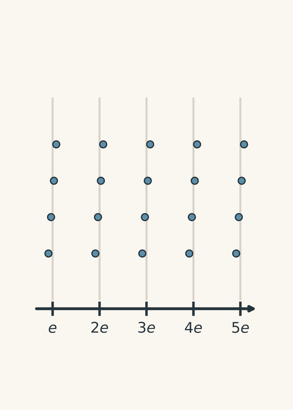
Suppose the measured magnitudes included values close to
\[ 1.6\times10^{-19}\ \text{C}, \]
\[ 3.2\times10^{-19}\ \text{C}, \]
\[ 4.8\times10^{-19}\ \text{C}, \]
and
\[ 8.0\times10^{-19}\ \text{C}. \]
These can be written as
\[ e,\quad 2e,\quad 3e,\quad 5e. \]
The charges are different, but they share a common smallest unit.
This is charge quantisation:
\[ q=ne, \]
where \(n\) is an integer and \(e\) is the magnitude of the elementary charge.
The oil droplets did not all have the same charge. That would actually have been less informative. Their different charges exposed the repeated unit underneath them.
Think of finding several shopping receipts with totals of $12, $20, $28, and $36, then discovering that every item costs $4. The totals differ, but the common step reveals the unit. The analogy breaks because electric charge is not literally assembled by buying identical objects one at a time in the experiment; it simply helps picture why several different measurements can reveal a common increment.
08What the result showed about electrons
The measured elementary charge is approximately
\[ e=1.602\times10^{-19}\ \text{C}. \]
An electron has charge
\[ q_e=-e=-1.602\times10^{-19}\ \text{C}. \]
The minus sign describes the type of charge. The value \(e\) itself conventionally means the positive magnitude of the elementary charge.
A proton has charge \(+e\).
So if an oil drop has charge
\[ q=-6.41\times10^{-19}\ \text{C}, \]
then
\[ \frac{|q|}{e} \approx \frac{6.41\times10^{-19}} {1.602\times10^{-19}} \approx4.00. \]
The drop therefore has four excess electrons, subject to measurement uncertainty.
Notice the wording: four excess electrons. The droplet contains vastly more than four electrons in total. Its negative charge means it contains four more electrons than would be required for electrical neutrality.
09Worked example: using several measurements to infer \(e\)
Four oil droplets are measured to have charge magnitudes
\[ 3.18\times10^{-19}\ \text{C},\quad 4.82\times10^{-19}\ \text{C},\quad 6.39\times10^{-19}\ \text{C},\quad 8.03\times10^{-19}\ \text{C}. \]
Estimate the elementary charge and identify the likely number of elementary charges on each droplet.
Step 1
The measurements are close to multiples of approximately \(1.60\times10^{-19}\) C.
Step 2
For \(e\approx1.60\times10^{-19}\) C:
\[ 2e\approx3.20\times10^{-19}\ \text{C}, \]
\[ 3e\approx4.80\times10^{-19}\ \text{C}, \]
\[ 4e\approx6.40\times10^{-19}\ \text{C}, \]
and
\[ 5e\approx8.00\times10^{-19}\ \text{C}. \]
The observations fit these values closely.
Step 3
\[ \frac{3.18\times10^{-19}}{2} =1.59\times10^{-19}\ \text{C}, \]
\[ \frac{4.82\times10^{-19}}{3} =1.607\times10^{-19}\ \text{C}, \]
\[ \frac{6.39\times10^{-19}}{4} =1.598\times10^{-19}\ \text{C}, \]
\[ \frac{8.03\times10^{-19}}{5} =1.606\times10^{-19}\ \text{C}. \]
These cluster near
\[ e\approx1.60\times10^{-19}\ \text{C}. \]
Step 4
The droplets most likely carry \(2e\), \(3e\), \(4e\), and \(5e\), respectively.
The slight mismatches are expected in real measurements. Quantisation does not mean every experimental result lands perfectly on an integer multiple before uncertainties are considered.
10Millikan did not directly measure the electron’s mass
This distinction is important.
Millikan’s experiment measured the elementary charge. It did not weigh an electron.
The electron’s mass became available because Thomson had already measured its charge-to-mass ratio.
Cathode-ray deflection experiments gave approximately
\[ \frac{e}{m_e}=1.76\times10^{11}\ \text{C kg}^{-1}, \]
where \(m_e\) is the electron mass.
If \(e\) is now known, rearrange:
\[ m_e=\frac{e}{e/m_e}. \]
Substituting,
\[ m_e= \frac{1.602\times10^{-19}\ \text{C}} {1.76\times10^{11}\ \text{C kg}^{-1}}. \]
Therefore,
\[ m_e\approx9.10\times10^{-31}\ \text{kg}. \]
The coulomb units cancel, leaving kilograms.
This is a good example of two experiments answering different halves of one problem:
| Experiment | What it established |
|---|---|
| Thomson’s cathode-ray work | The electron’s charge-to-mass ratio, \(e/m_e\) |
| Millikan’s oil-drop experiment | The elementary charge, \(e\) |
| Combined result | Electron mass, \(m_e\) |
If Thomson’s experiment is still fuzzy, review cathode-ray evidence for electrons before memorising this chain. The logic matters more than remembering two surnames.
11Worked example: finding the electron mass
An experiment gives the electron charge-to-mass ratio as
\[ \frac{e}{m_e}=1.76\times10^{11}\ \text{C kg}^{-1}. \]
Use \(e=1.60\times10^{-19}\) C to calculate the electron mass.
Step 1
We know \(e\) and \(e/m_e\), and we want \(m_e\).
Step 2
\[ m_e=\frac{e}{e/m_e}. \]
Step 3
\[ m_e= \frac{1.60\times10^{-19}\ \text{C}} {1.76\times10^{11}\ \text{C kg}^{-1}} =9.09\times10^{-31}\ \text{kg}. \]
Step 4
The electron mass is about
\[ 9.1\times10^{-31}\ \text{kg}. \]
Neither Thomson’s measurement nor Millikan’s measurement alone gives this result. It emerges by combining them.
12What changed when the drop gained or lost an electron?
One especially useful feature of the experiment was that the charge on an individual droplet could sometimes change while the droplet itself remained under observation.
Suppose the mass stays essentially constant but the charge changes from \(3e\) to \(4e\).
For suspension,
\[ qE=mg. \]
Because \(m\) and \(g\) have not changed,
\[ E=\frac{mg}{q}. \]
Increasing the magnitude of \(q\) therefore means a smaller electric field is needed to suspend the same drop.
For the parallel plates,
\[ E=\frac{V}{d}. \]
If \(d\) is fixed, the balancing voltage also decreases.
A student might predict the opposite: “More charge means stronger electric force, so we need more voltage.” The first half is correct. More charge does mean more electric force at the same field. That is exactly why less field is required to produce the same upward force.
For one unchanged droplet,
\[ q_1E_1=q_2E_2. \]
So if its charge changes from \(3e\) to \(4e\),
\[ 3eE_1=4eE_2, \]
giving
\[ E_2=\frac34E_1. \]
That kind of reasoning is more useful than treating \(qE=mg\) as a formula into which numbers are mechanically dropped.
13Why Brownian motion and tiny-drop physics mattered
Making a droplet smaller has an apparent advantage: its weight becomes tiny, so the electric force needed to control it also becomes tiny.
But smaller is not automatically better.
Microscopic droplets are constantly struck by air molecules. Those molecular collisions contribute to irregular Brownian motion. The smaller the object, the more noticeable this random motion becomes compared with its smooth gravitational motion.
So there is a measurement trade-off.
Large drops fall faster and are less dominated by Brownian motion, but require greater electric forces. Very small drops are easier to influence electrically, but their motion is harder to measure cleanly.
There is another complication. Ordinary Stokes’ law treats the surrounding air as a continuous fluid. For extremely small droplets, that approximation becomes imperfect because the scale of the droplet begins to matter relative to molecular motion in the gas. A correction is then required.
For HSC Physics, you normally do not need to reproduce the full correction mathematics. You do need to understand the experimental principle: the simple force equations describe the core model, while precision measurement requires corrections for effects that the ideal model leaves out.
14What evidence actually supports quantisation?
It is tempting to say, “Millikan got \(1.6\times10^{-19}\) C, therefore charge is quantised.”
That skips the strongest part of the reasoning.
Quantisation is supported by the pattern across many measurements.
If charge were freely continuous, measurements could in principle appear at arbitrary values such as
\[ 2.37\times10^{-19}\ \text{C} \]
or
\[ 5.11\times10^{-19}\ \text{C} \]
without lining up with any common unit.
Instead, measured droplet charges clustered around integer multiples of a common value.
The important evidence is therefore not merely a particular number. It is the repeated structure
\[ q=ne. \]
Experimental uncertainty makes the measured values fuzzy. The integer pattern is recovered by asking whether the data are consistent with multiples of one common charge.
15Observation, interpretation, and modern hindsight
It helps to separate three layers.
The observation was that different droplets required particular electric fields to balance their weight, and the inferred charges occurred in a repeated numerical pattern.
The interpretation was that electric charge exists in discrete units rather than arbitrary amounts.
Modern hindsight connects that unit directly with the charge magnitude carried by a proton or electron:
\[ e=1.602176634\times10^{-19}\ \text{C}. \]
The coulomb is now defined within the SI system using an exact numerical value for the elementary charge. Millikan, of course, was not verifying a modern definition. His experiment belonged to an earlier stage of physics, when the value and discreteness of elementary charge were experimental questions.
16What an HSC answer should and should not claim
If asked about Millikan’s contribution, a strong answer should distinguish between what he measured and what could later be calculated.
A compact causal chain is:
\[ \text{droplet motion} \rightarrow \text{droplet size and mass} \rightarrow \text{electric force balance} \rightarrow \text{droplet charge} \rightarrow \text{common elementary charge}. \]
Then:
\[ e + \frac{e}{m_e} \rightarrow m_e. \]
Avoid these common mistakes:
| Tempting statement | What is wrong with it? |
|---|---|
| “Millikan measured the mass of an electron.” | He measured elementary charge; electron mass was calculated using Thomson’s \(e/m\). |
| “The electric force made gravity disappear.” | Gravity still acted. The forces balanced. |
| “Every oil drop had charge \(e\).” | Drops could carry \(e\), \(2e\), \(3e\), and other integer multiples. |
| “A drop with charge \(-3e\) contains three electrons.” | It has three excess electrons, not three electrons in total. |
| “One measured charge proves quantisation.” | The evidence comes from a pattern across many measurements. |
| “A stationary drop has no forces acting on it.” | Its net force is zero; individual forces are still present. |
17Questions and solutions
Question 1
An oil drop of mass \(3.2\times10^{-15}\) kg is held stationary in a vertical electric field of magnitude \(9.8\times10^4\ \text{N C}^{-1}\).
Take \(g=9.8\ \text{m s}^{-2}\).
Calculate:
a. the magnitude of the charge on the drop, and
b. the number of excess electrons if the drop is negatively charged.
Use \(e=1.60\times10^{-19}\) C.
Solution 1
The drop has charge magnitude \(3.2\times10^{-19}\) C, corresponding to two excess electrons.
Because the drop is stationary, its acceleration is zero and the upward electric force balances its weight:
\[ qE=mg. \]
Rearranging,
\[ q=\frac{mg}{E}. \]
Substitute:
\[ q= \frac{(3.2\times10^{-15}\ \text{kg})(9.8\ \text{m s}^{-2})} {9.8\times10^4\ \text{N C}^{-1}} =3.2\times10^{-19}\ \text{C}. \]
Now compare this with the elementary charge:
\[ n= \frac{q}{e} = \frac{3.2\times10^{-19}} {1.60\times10^{-19}} =2. \]
So a negatively charged drop has two excess electrons.
A common trap is to write that the drop “contains two electrons”. It contains an enormous number of electrons. Its net negative charge corresponds to two electrons beyond the neutral number.
Question 2
A negatively charged oil drop is held stationary between two parallel horizontal plates separated by \(5.0\times10^{-3}\) m. The potential difference across the plates is \(600\) V.
The droplet has mass \(8.2\times10^{-15}\) kg.
a. Calculate the electric field magnitude.
b. Calculate the magnitude of the droplet’s charge.
c. Estimate the number of excess electrons.
Use \(g=9.8\ \text{m s}^{-2}\) and \(e=1.60\times10^{-19}\) C.
Solution 2
The field is \(1.2\times10^5\ \text{N C}^{-1}\), and the droplet carries about \(6.7\times10^{-19}\) C, which is consistent with approximately four elementary charges once realistic measurement uncertainty is considered.
For parallel plates,
\[ E=\frac{V}{d}. \]
Substituting,
\[ E= \frac{600\ \text{V}} {5.0\times10^{-3}\ \text{m}} =1.2\times10^5\ \text{V m}^{-1}. \]
Since \(1\ \text{V m}^{-1}=1\ \text{N C}^{-1}\),
\[ E=1.2\times10^5\ \text{N C}^{-1}. \]
For suspension,
\[ qE=mg, \]
so
\[ q=\frac{mg}{E}. \]
Substitute:
\[ q= \frac{(8.2\times10^{-15})(9.8)} {1.2\times10^5} =6.70\times10^{-19}\ \text{C}. \]
The apparent number of elementary charges is
\[ n= \frac{6.70\times10^{-19}} {1.60\times10^{-19}} \approx4.19. \]
An exact charge of \(4e\) would be
\[ 4e=6.40\times10^{-19}\ \text{C}. \]
The calculated value does not land exactly on an integer because the given experimental quantities have finite precision and because the simplified force model ignores effects such as buoyancy.
The tempting route is to treat \(4.19\) as meaning “4.19 electrons”. That is not the physical interpretation. A single droplet should carry an integer multiple of \(e\); non-integer experimental ratios signal uncertainty, modelling limitations, or measurement error rather than fractional ordinary electrons on the drop.
Question 3
A particular oil drop is initially stationary when the electric field magnitude is \(E_1=8.0\times10^4\ \text{N C}^{-1}\). While the same drop remains under observation, it gains one additional electron.
It is then stationary at \(E_2=6.0\times10^4\ \text{N C}^{-1}\).
Assume its mass does not change appreciably.
Determine the initial magnitude of the charge on the drop in units of \(e\).
Solution 3
The initial charge magnitude was \(3e\), and after gaining one electron its magnitude was \(4e\).
For the same stationary drop,
\[ qE=mg. \]
The mass and gravitational field are unchanged, so the balancing product \(qE\) is the same before and after the extra electron is acquired.
Let the original magnitude of charge be \(ne\). After gaining one electron, its magnitude becomes \((n+1)e\).
Therefore,
\[ neE_1=(n+1)eE_2. \]
Cancel \(e\):
\[ nE_1=(n+1)E_2. \]
Substitute the field strengths:
\[ n(8.0\times10^4) = (n+1)(6.0\times10^4). \]
Cancelling \(10^4\),
\[ 8n=6n+6. \]
Thus,
\[ 2n=6, \]
so
\[ n=3. \]
The initial charge magnitude was therefore
\[ 3e. \]
After gaining the extra electron, it became \(4e\).
A tempting prediction is that gaining charge should require a stronger balancing field. The opposite is true. Since \(F_E=qE\), a larger charge needs a smaller field to provide the same upward force.
This type of measurement is especially powerful because the droplet’s unknown mass cancels. Watching the same droplet before and after a one-electron charge change can reveal integer charge relationships without first needing its mass.
Question 4
Two groups analyse the same oil-drop data.
Group A says:
“The measured charges are \(3.21\), \(4.78\), \(6.42\), and \(8.01\), all in units of \(10^{-19}\) C. These are nearly multiples of \(1.60\times10^{-19}\) C, so \(e\approx1.60\times10^{-19}\) C.”
Group B replies:
“They are also nearly multiples of \(0.80\times10^{-19}\) C: approximately \(4\), \(6\), \(8\), and \(10\) units. Therefore the experiment cannot distinguish \(e=1.60\times10^{-19}\) C from \(e=0.80\times10^{-19}\) C.”
Is Group B’s argument logically valid from those four measurements alone? Explain what additional evidence would be needed to decide whether \(1.60\times10^{-19}\) C is actually the elementary unit.
Solution 4
Group B has identified a real logical limitation: those four measurements alone do not prove that \(1.60\times10^{-19}\) C is the smallest possible unit.
The measured values are approximately
\[ 3.2,\ 4.8,\ 6.4,\ 8.0 \]
in units of \(10^{-19}\) C.
They fit
\[ 2e,\ 3e,\ 4e,\ 5e \]
if
\[ e=1.60\times10^{-19}\ \text{C}. \]
But they can also be written approximately as
\[ 4e',\ 6e',\ 8e',\ 10e' \]
if
\[ e'=0.80\times10^{-19}\ \text{C}. \]
So these four values establish a common spacing pattern but do not, by themselves, prove that the larger proposed unit is indivisible.
The key extra evidence would be measurements of drops carrying odd multiples of \(0.80\times10^{-19}\) C if that smaller quantity were the true elementary charge.
For example, a reliably measured charge near
\[ 1.60\times10^{-19}\ \text{C} \]
still would not distinguish the models, because it equals \(2e'\).
But a stable charge near
\[ 0.80\times10^{-19}\ \text{C}, \]
\[ 2.40\times10^{-19}\ \text{C}, \]
or another odd multiple of \(0.80\times10^{-19}\) C would support the smaller unit.
If sufficiently sensitive measurements repeatedly show charges at
\[ 1.60,\ 3.20,\ 4.80,\ 6.40,\ldots \]
times \(10^{-19}\) C but never at the halfway values allowed by the \(0.80\times10^{-19}\) C hypothesis, then the smaller proposed unit loses support.
The tempting route is to say, “Take the greatest common factor of the numbers.” Real measurements are not exact integers, and a mathematical common factor can always be made smaller. Experimental quantisation requires more than finding some number that divides the measurements approximately. It requires evidence that charge changes occur in a smallest observed increment and that allowed intermediate values are absent within the experiment’s resolution.
This is why a large collection of measurements, especially observations of individual drops changing charge in discrete steps, is much stronger than a short table of convenient multiples.
Question 5
An oil drop of unknown mass is stationary in an upward electric force when its negative charge has magnitude \(5e\). Its balancing electric field has magnitude \(E_1\).
The drop then loses one electron. Before the field is adjusted, it begins to move downward. The experimenter increases the electric field until the drop is stationary again at field \(E_2\).
A student argues:
“Because the drop moved downward, gravity must have become stronger. Therefore this observation cannot tell us anything about charge quantisation unless we already know the mass.”
Another student argues:
“The mass is unnecessary. The two balance conditions alone can test whether the charge changed by exactly one elementary unit.”
Assume the loss of one electron makes a negligible change to the droplet’s total mass.
a. Determine \(E_2/E_1\).
b. Explain why the downward motion immediately after the electron was lost is expected.
c. Show how a sequence of balancing-field measurements on the same unknown droplet could provide evidence for quantised charge even without determining its mass.
d. State the conceptual limitation: why would ratios of balancing fields alone still not establish the numerical value of \(e\) in coulombs?
Solution 5
The second student is correct: \(E_2/E_1=5/4\), and repeated balancing-field ratios for the same droplet can reveal integer charge changes without knowing its mass. However, those ratios alone cannot determine the size of \(e\) in coulombs.
Initially the charge magnitude is
\[ q_1=5e. \]
Because the drop is stationary,
\[ 5eE_1=mg. \]
After one electron is lost, the negative charge magnitude becomes
\[ q_2=4e. \]
For the drop to be stationary again,
\[ 4eE_2=mg. \]
Since both expressions equal the same \(mg\),
\[ 5eE_1=4eE_2. \]
Cancel \(e\):
\[ 5E_1=4E_2. \]
Therefore,
\[ \frac{E_2}{E_1}=\frac54=1.25. \]
The required electric field must increase by 25%.
Immediately after the electron is lost, however, the field is still \(E_1\). The upward electric force therefore changes from
\[ F_{E,\text{before}}=5eE_1 \]
to
\[ F_{E,\text{after}}=4eE_1. \]
But gravity is still
\[ mg=5eE_1. \]
Therefore,
\[ F_{E,\text{after}}<mg. \]
The net force is downward, so the droplet begins to accelerate downward.
Gravity has not become stronger. The upward electric force has become weaker because the magnitude of the charge decreased.
Now consider why repeated measurements on the same droplet are so useful. For every stationary state,
\[ q_iE_i=mg. \]
If the drop’s mass remains constant,
\[ q_i\propto\frac{1}{E_i}. \]
Suppose successive charge states correspond to
\[ 5e,\quad4e,\quad3e,\quad2e. \]
Their balancing fields would satisfy
\[ 5eE_5=4eE_4=3eE_3=2eE_2=mg. \]
So the field magnitudes would be proportional to
\[ \frac15,\quad\frac14,\quad\frac13,\quad\frac12. \]
Ratios between measured fields could therefore reveal simple integer relationships among charge states without requiring \(m\).
This defeats the first student’s argument. The unknown gravitational force is not an obstacle when comparing multiple balanced states of the same droplet because the same \(mg\) appears in every equation and cancels.
The harder limitation appears in part d.
Suppose the experiment shows convincingly that the droplet passes through states whose charges have relative magnitudes
\[ 2:3:4:5. \]
That establishes a discrete pattern. But the balancing-field ratios contain no absolute charge scale. The equations could involve
\[ 2e,\ 3e,\ 4e,\ 5e \]
for one value of \(e\), or
\[ 2k,\ 3k,\ 4k,\ 5k \]
for another unknown unit \(k\), and the field ratios would be identical.
To determine the numerical value of the elementary charge in coulombs, an absolute force measurement is needed. That requires knowing quantities such as the droplet’s effective weight and electric field magnitude, not merely ratios between charge states.
The conceptual hinge is that quantisation and calibration are different achievements.
Repeated measurements on one droplet can reveal that charge changes in discrete steps. Determining that each step is specifically about
\[ 1.60\times10^{-19}\ \text{C} \]
requires an independently calibrated measurement scale.
That distinction links Millikan’s work back to Thomson’s. Thomson established a charge-to-mass ratio; Millikan supplied an absolute charge scale. Together, those measurements converted a pattern of cathode-ray behaviour into numerical properties of the electron itself.