
Point Charges vs Parallel Plates: Choosing the Right Field Model
Learn why electric fields weaken with distance around a point charge but remain approximately uniform between parallel plates. Compare the two equations, understand what each distance represents, and practise with worked examples and challenging HSC-style questions.
At 10 cm from a small charged sphere, the electric field has a particular strength. Move twice as far from its centre, and the field drops to one-quarter of its original value. But between two large parallel plates, moving a test charge across the central gap leaves the field approximately unchanged.
Both situations involve electric fields. So why does the field weaken with distance in one case but not the other?
Predict before reading on: if a distance doubles, does the electric field always halve? No. The answer depends on what creates the field and what the distance in your equation actually represents.
Two electric-field patterns
| Positive point charge | E = k|q|/r² Radial field lines point away from the charge and spread farther apart with distance. |
|---|---|
| Parallel plates | E ≈ V/d Field lines are straight, parallel, and evenly spaced in the central gap; they fringe near the edges. |
The diagrams give you the first clue. Around a point charge, the field spreads out in all directions. Between parallel plates, the field is approximately uniform across the central region.
These are two different field patterns, so they require two different models.
01The point-charge model: field strength falls with distance
Imagine placing a small positive test charge near an isolated charged particle. The particle experiences an electric force.
Move the test charge farther away. The force becomes weaker.
For an isolated point charge, the field strength decreases according to the inverse-square relationship:
\[ E=\frac{k|q|}{r^2} \]
Here:
- \(E\) is the electric-field strength, measured in newtons per coulomb (\(\text{N C}^{-1}\)).
- \(k\) is Coulomb’s constant, approximately \(8.99\times10^9\ \text{N m}^2\text{C}^{-2}\).
- \(q\) is the source charge, measured in coulombs (C).
- \(r\) is the distance from the centre of the source charge to the point where you are calculating the field, measured in metres (m).
The absolute value, \(|q|\), gives the magnitude of the field. The sign of the source charge determines its direction.
A positive source charge produces a field directed away from it. A negative source charge produces a field directed towards it.
The same model also applies outside a spherically symmetric charged object, such as a charged conducting sphere, when its external field behaves like that of a point charge at its centre.
Why does the field follow an inverse-square relationship?
Picture the field spreading outwards from a point charge. At twice the distance, the field has spread across a spherical surface with four times the area. At three times the distance, that area is nine times as large.
The field becomes weaker as it spreads over this increasing area. Mathematically, the strength is proportional to \(1/r^2\).
This gives you a useful exam shortcut:
- Double \(r\): divide \(E\) by \(4\).
- Triple \(r\): divide \(E\) by \(9\).
- Halve \(r\): multiply \(E\) by \(4\).
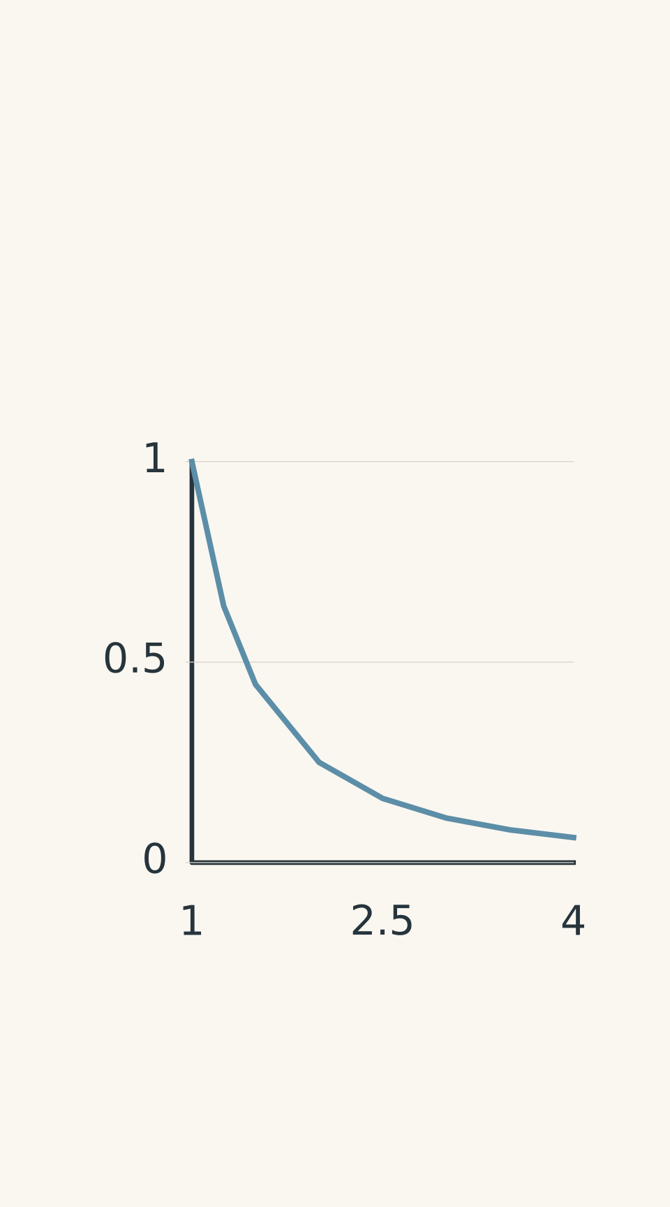
- Inverse-square relationship
Notice what the equation does not use: the distance from the surface of the charged object.
If a spherical object has a radius of 2 cm and your test point is 3 cm beyond its surface, then \(r=5\text{ cm}\), not 3 cm. The equation measures from the centre.
Worked example: Finding the field around a point charge
An isolated charge of \(+4.0\,\mu\text{C}\) produces an electric field at a point 0.30 m from its centre. Calculate the field strength and state its direction. Use \(k=8.99\times10^9\ \text{N m}^2\text{C}^{-2}\).
Step 1
The source is a point charge, so use the inverse-square equation.
\[ q=4.0\times10^{-6}\text{ C} \]
\[ r=0.30\text{ m} \]
Step 2
\[ \begin{aligned} E&=\frac{k|q|}{r^2}\\[4pt] &=\frac{(8.99\times10^9)(4.0\times10^{-6})}{(0.30)^2}\\[4pt] &=4.0\times10^5\ \text{N C}^{-1} \end{aligned} \]
Step 3
The source charge is positive, so the electric field points away from it.
The answer is \(4.0\times10^5\ \text{N C}^{-1}\), directed radially outwards.
If the point were moved from 0.30 m to 0.60 m, the field would fall to one-quarter of this value. You can predict that immediately without repeating the full calculation.
02The parallel-plate model: field strength is approximately uniform
Now consider two large, oppositely charged parallel plates.
Between the plates, the electric field is approximately uniform in the central region. Its magnitude and direction remain almost constant from one location to another.
The field lines are straight, parallel, and evenly spaced. Unlike the radial pattern around a point charge, they do not spread out from a single source.
The field strength is calculated using:
\[ E\approx\frac{V}{d} \]
Here:
- \(E\) is the electric-field strength, measured in \(\text{V m}^{-1}\) or \(\text{N C}^{-1}\).
- \(V\) is the magnitude of the potential difference between the plates, measured in volts (V).
- \(d\) is the perpendicular separation between the plates, measured in metres (m).
The symbol \(\approx\) reminds you that this is an approximation for the uniform-field region of real plates.
The relationship follows from the fact that, for a uniform field, the magnitude of the potential difference across a distance \(d\) is \(V=Ed\).
The important difference: what does the distance mean?
This is where students often mix up the two equations.
In the point-charge model, \(r\) measures the distance from the source charge to the point where you want the field.
In the parallel-plate model, \(d\) measures the gap between the plates. It does not measure how far your test charge is from the positive plate.
Which distance belongs in the equation?
| Point charge | E = k|q|/r² r: distance from the charge centre to the field point. Doubling r reduces E to one-quarter. |
|---|---|
| Parallel plates | E ≈ V/d d: full gap between plates; x: position of the test point within the gap. In the ideal central field, E is independent of x. |
Suppose you move a test charge from one location to another inside the same parallel-plate gap. If both locations are in the uniform-field region, the field strength stays approximately the same.
Why? Neither the plate separation nor the potential difference has changed.
Now imagine increasing the gap while keeping the potential difference fixed. The equation \(E\approx V/d\) tells you that the field becomes weaker as the gap increases.
These are two different changes:
- Moving a test charge inside a fixed gap does not change the ideal field strength.
- Increasing the gap at fixed voltage decreases the field strength.
Do not confuse the position of the test charge with the separation of the plates.
What happens near the edges?
The parallel-plate model is not exact everywhere. Near the edges, the field lines bend outwards. This is called fringing.
The approximation \(E\approx V/d\) works best when the plates are large compared with their separation and you are considering the central region.
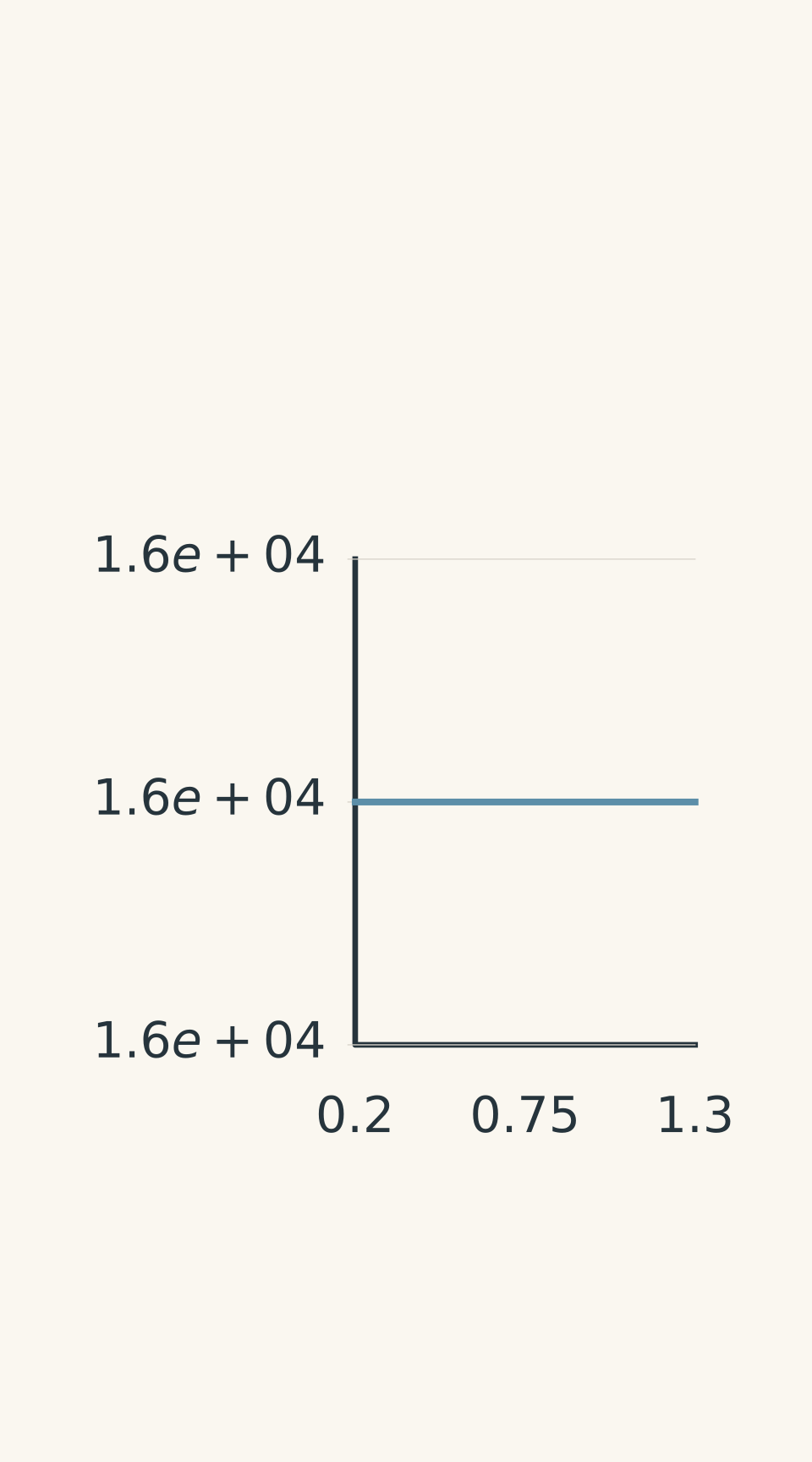
- Central uniform-field region; edges excluded
Worked example: Calculating the field between parallel plates
Two large parallel plates have a potential difference of 240 V and a separation of 1.5 cm. Calculate the electric-field strength in the central region. Then determine the force on a \(+3.0\,\text{nC}\) charge placed there.
Step 1
The source geometry is a pair of parallel plates, so use \(E\approx V/d\).
\[ d=1.5\text{ cm}=0.015\text{ m} \]
Step 2
\[ \begin{aligned} E&\approx\frac{V}{d}\\[4pt] &=\frac{240}{0.015}\\[4pt] &=1.6\times10^4\ \text{V m}^{-1} \end{aligned} \]
Therefore, the field strength is approximately \(1.6\times10^4\ \text{N C}^{-1}\).
Step 3
Electric-field strength is force per unit charge:
\[ E=\frac{F}{q_{\text{test}}} \]
Rearrange to find the force:
\[ F=q_{\text{test}}E \]
The test charge is \(3.0\times10^{-9}\text{ C}\), so
\[ \begin{aligned} F&=(3.0\times10^{-9})(1.6\times10^4)\\[4pt] &=4.8\times10^{-5}\text{ N} \end{aligned} \]
The force has a magnitude of \(4.8\times10^{-5}\text{ N}\) and points towards the negative plate.
Notice that the test charge’s position does not appear in the field equation. Provided it remains in the uniform-field region, the field strength is approximately constant.
03Choosing the correct equation
Both equations calculate electric-field strength, but they describe different physical situations.
| Feature | Point-charge model | Parallel-plate model |
|---|---|---|
| Equation | \(E=k|q|/r^2\) | \(E\approx V/d\) |
| Source | An isolated point charge | Large, oppositely charged parallel plates |
| Distance | \(r\), from the charge centre to the field point | \(d\), the gap between plates |
| Field pattern | Radial | Approximately uniform in the central region |
| Effect of moving the field point | Strength changes with \(1/r^2\) | Strength stays approximately constant within the uniform region |
| Main limitation | Requires point-charge or suitable spherical symmetry | Becomes less accurate near plate edges |
Choose the correct electric-field model
- Identify the source geometry
Isolated point charge or suitable spherical symmetry; or large parallel plates?
- Select the equation
Point charge: E = k|q|/r²
Parallel plates: E ≈ V/dMatch the equation to the source geometry.
- Check the distance
r: charge centre to field point.
d: full separation between plates.
- Check for plate-edge effects
Near plate edges, fringing occurs and the uniform-field approximation may fail. This check applies to the parallel-plate model.
Use this decision rule when you see an unfamiliar exam question:
- Identify what produces the field.
- Identify the information given: source charge and distance, or plate voltage and separation.
- Choose the matching equation, convert all distances to metres, and check the field’s direction separately.
The units can help you check your calculation. Both \(\text{N C}^{-1}\) and \(\text{V m}^{-1}\) are valid units for electric-field strength.
One further caution: if a point charge and parallel plates both contribute to the field at a location, neither equation alone gives the total field. You must calculate the contributions separately and add them as vectors.
04Questions and solutions
Question 1
Two large parallel plates have a potential difference of 180 V and a separation of 3.0 cm. Estimate the electric-field strength in the central region and state its direction.
Solution 1
The field strength is approximately \(6.0\times10^3\ \text{N C}^{-1}\), directed from the positive plate towards the negative plate.
The plates are large and parallel, so the uniform-field approximation applies. First, convert the separation:
\[ d=3.0\text{ cm}=0.030\text{ m} \]
Then use the plate equation:
\[ \begin{aligned} E&\approx\frac{V}{d}\\[4pt] &=\frac{180}{0.030}\\[4pt] &=6.0\times10^3\ \text{V m}^{-1} \end{aligned} \]
The field points from the positive plate to the negative plate. The result is a field magnitude, so the direction must be stated separately.
Question 2
An isolated positive point charge of \(+6.0\,\mu\text{C}\) produces an electric field.
(a) Calculate the field strength at a distance of 0.20 m from its centre.
(b) Calculate the field strength at a distance of 0.40 m from its centre.
(c) A positive test charge of \(+2.0\,\text{nC}\) is placed at 0.40 m. Calculate the force on it and state the direction.
Use \(k=8.99\times10^9\ \text{N m}^2\text{C}^{-2}\).
Solution 2
The field at 0.40 m is one-quarter of the field at 0.20 m, and the test charge experiences a force of approximately \(6.7\times10^{-4}\text{ N}\), directed away from the source charge.
(a) At \(r=0.20\text{ m}\), use the inverse-square equation:
\[ \begin{aligned} E_1&=\frac{k|q|}{r^2}\\[4pt] &=\frac{(8.99\times10^9)(6.0\times10^{-6})}{(0.20)^2}\\[4pt] &=1.35\times10^6\ \text{N C}^{-1} \end{aligned} \]
To two significant figures,
\[ E_1=1.3\times10^6\ \text{N C}^{-1} \]
(b) At \(r=0.40\text{ m}\),
\[ \begin{aligned} E_2&=\frac{(8.99\times10^9)(6.0\times10^{-6})}{(0.40)^2}\\[4pt] &=3.37\times10^5\ \text{N C}^{-1}\\[4pt] &\approx3.4\times10^5\ \text{N C}^{-1} \end{aligned} \]
The distance has doubled, so the field has fallen to one-quarter of its original value:
\[ \frac{E_2}{E_1}=\frac{1}{4} \]
The tempting mistake is to halve the field because the distance doubled. The distance is squared in the denominator, so the field falls by a factor of four.
(c) Use \(F=q_{\text{test}}E\):
\[ \begin{aligned} F&=(2.0\times10^{-9})(3.37\times10^5)\\[4pt] &=6.74\times10^{-4}\text{ N}\\[4pt] &\approx6.7\times10^{-4}\text{ N} \end{aligned} \]
Both charges are positive, so the force on the test charge is repulsive and directed away from the source.
Question 3
Two large parallel plates are connected to a power supply that maintains a constant potential difference of 300 V.
The plate separation increases from 1.0 cm to 2.5 cm.
(a) Calculate the initial and final electric-field strengths in the central region.
(b) An electron remains in the central region after the gap has increased. Calculate the magnitude of the electric force on it and state the force’s direction.
Use the magnitude of the electron’s charge, \(1.60\times10^{-19}\text{ C}\).
Solution 3
The field decreases from \(3.0\times10^4\ \text{N C}^{-1}\) to \(1.2\times10^4\ \text{N C}^{-1}\). The electron experiences a force of \(1.9\times10^{-15}\text{ N}\), directed towards the positive plate.
(a) Initially,
\[ d_1=1.0\text{ cm}=0.010\text{ m} \]
Therefore,
\[ \begin{aligned} E_1&\approx\frac{300}{0.010}\\[4pt] &=3.0\times10^4\ \text{V m}^{-1} \end{aligned} \]
After the separation increases,
\[ d_2=2.5\text{ cm}=0.025\text{ m} \]
The new field is
\[ \begin{aligned} E_2&\approx\frac{300}{0.025}\\[4pt] &=1.2\times10^4\ \text{V m}^{-1} \end{aligned} \]
The field has decreased because the voltage remains fixed while the plate separation increases.
(b) The force magnitude is
\[ |F|=|q_{\text{test}}|E \]
Substituting the final field strength,
\[ \begin{aligned} |F|&=(1.60\times10^{-19})(1.2\times10^4)\\[4pt] &=1.92\times10^{-15}\text{ N}\\[4pt] &\approx1.9\times10^{-15}\text{ N} \end{aligned} \]
The electric field points from the positive plate to the negative plate. An electron is negatively charged, so the force on it points in the opposite direction, towards the positive plate.
The key condition is that the voltage is held constant. If the voltage were allowed to change, you could not assume the same relationship between the change in gap and the change in field.
Question 4
Two large parallel plates are separated by 4.0 cm and have a potential difference of 200 V. Points A and B are both in the uniform-field region. Point A is 0.5 cm from the positive plate, while point B is 2.0 cm from the positive plate.
A student argues that the field at B must be one-sixteenth of the field at A because B is four times farther from the positive plate.
(a) Evaluate the student’s claim and calculate the field at each point.
(b) If A and B were instead at distances of 0.5 cm and 2.0 cm from an isolated point charge, what would the ratio \(E_B/E_A\) be?
Explain why the same change in distance produces different results in the two situations.
Solution 4
The student’s claim is incorrect for the parallel plates: both points have a field strength of approximately \(5.0\times10^3\ \text{N C}^{-1}\). For a point charge at the stated distances, the field at B would be one-sixteenth of the field at A.
(a) For the plates, the relevant distance is the full plate separation:
\[ d=4.0\text{ cm}=0.040\text{ m} \]
Therefore,
\[ \begin{aligned} E&\approx\frac{V}{d}\\[4pt] &=\frac{200}{0.040}\\[4pt] &=5.0\times10^3\ \text{N C}^{-1} \end{aligned} \]
Both points are in the uniform-field region, so
\[ E_A\approx E_B\approx5.0\times10^3\ \text{N C}^{-1} \]
The distance from the positive plate to the test point does not determine the field strength in this model.
(b) For a point charge, the field depends on the square of the distance from the charge’s centre:
\[ \frac{E_B}{E_A} =\frac{r_A^2}{r_B^2} \]
Substitute the two distances. Their units cancel in the ratio:
\[ \begin{aligned} \frac{E_B}{E_A} &=\left(\frac{0.5}{2.0}\right)^2\\[4pt] &=\frac{1}{16} \end{aligned} \]
The field at B is one-sixteenth of the field at A.
The important distinction is that the point-charge equation uses the distance from the source to the field point, while the parallel-plate equation uses the fixed gap between the plates. The equations describe different spatial patterns, even when the distances happen to have the same ratio.
Question 5
Two identical positive test particles have the same charge \(q_{\text{test}}\) and mass \(m\). Both are released from rest.
At their starting points, the electric-field magnitude is
\[ E_0=2.0\times10^4\ \text{N C}^{-1} \]
Particle A starts \(r_0=0.10\text{ m}\) from an isolated positive point charge and moves directly away from it.
Particle B starts in the central region between large parallel plates. The plate voltage and separation satisfy \(V/d=E_0\). The gap is wide enough that B remains in the uniform-field region as it moves.
Both particles travel 0.10 m along the direction of the electric field.
(a) Compare their initial accelerations.
(b) Calculate the electric-field magnitude acting on each particle after the 0.10 m displacement. Hence, compare their accelerations at that instant.
(c) A student concludes that B must be moving four times as fast as A because B has four times the acceleration at the end of the displacement. Evaluate this claim. Which particle is faster, and what further reasoning is needed to compare their speeds quantitatively?
Ignore gravity and all other forces.
Solution 5
The particles have the same initial acceleration. After moving 0.10 m, B has four times A’s acceleration. B is also moving faster, but a fourfold difference in acceleration does not imply a fourfold difference in speed.
(a) Initial accelerations
Electric-field strength is force per unit charge:
\[ E=\frac{F}{q_{\text{test}}} \]
Using Newton’s second law, \(F=ma\), gives
\[ a=\frac{q_{\text{test}}E}{m} \]
Both particles have the same charge, mass, and initial field magnitude. Therefore,
\[ a_{A,0}=a_{B,0}=\frac{q_{\text{test}}E_0}{m} \]
Their initial accelerations are equal.
This tells us what happens at the instant of release. It does not tell us that their fields will remain equal as they move.
(b) Fields and accelerations after the displacement
Particle A moves away from the point charge, increasing its distance from \(r_0=0.10\text{ m}\) to
\[ r=0.10+0.10=0.20\text{ m}=2r_0 \]
The point-charge field therefore becomes
\[ \begin{aligned} E_A&=E_0\left(\frac{r_0}{2r_0}\right)^2\\[4pt] &=\frac{E_0}{4}\\[4pt] &=5.0\times10^3\ \text{N C}^{-1} \end{aligned} \]
Particle B remains in the central region between the plates, so its field remains approximately uniform:
\[ E_B\approx E_0=2.0\times10^4\ \text{N C}^{-1} \]
The field ratio is
\[ \frac{E_B}{E_A} =\frac{2.0\times10^4}{5.0\times10^3} =4 \]
Since the particles have identical charge and mass, their accelerations have the same ratio as their field magnitudes:
\[ \frac{a_B}{a_A}\approx4 \]
Particle B’s acceleration is four times A’s acceleration at that instant.
(c) Does four times the acceleration mean four times the speed?
No. Acceleration describes how quickly velocity changes at a particular instant. Speed depends on the accumulated effect of the force throughout the motion.
At the start, the particles experience equal forces. As they move, however, A’s field weakens while B’s field stays approximately constant. After any positive displacement, B experiences a greater force than A.
Both forces act along the direction of motion, so the electric field does more work on B over the same displacement. Starting from rest, B therefore gains more kinetic energy and reaches a greater speed.
However, the final acceleration ratio alone does not tell you the speed ratio. To calculate their speeds quantitatively, you must compare the work done over the entire path, using the changing field for A and the approximately constant field for B.
This is the crucial distinction: equal field strengths at one location do not mean the fields behave identically everywhere else. The source geometry determines how the field changes, which then affects the motion.
Once you can choose the correct field model, the next step is predicting how charged particles respond to it. Use \(F=q_{\text{test}}E\) to find the instantaneous force, then use work and energy when the field changes along a particle’s path. That is where the difference between a radial field and a uniform field becomes especially useful.