
Circular Motion Investigations: HSC Physics Practice Exam
Test your understanding of circular motion investigations with this original, timed Physics practice paper. Includes 50 marks of questions on experimental data, graph analysis, uncertainty, and force relationships, followed by complete worked solutions and a marking guide.
This original tutorgum practice paper assesses how experimental evidence can be used to test the relationships between centripetal force, mass, speed, radius, and period in uniform circular motion. It covers only the circular-motion-investigations scope for the Physics 2017 syllabus edition. It is a focused topic assessment, not a full-course exam or an official, endorsed, past, or predicted NESA paper.
01Exam instructions
| Assessment condition | Details |
|---|---|
| Suggested reading time | 5 minutes |
| Suggested working time | 75 minutes |
| Total marks | 50 |
| Permitted equipment | Scientific calculator, ruler, pencil, and graph paper |
| Formula sheet | Not supplied |
Assessed content
This paper assesses your ability to:
- Use \(a_c = v^2/r\) to calculate centripetal acceleration and explain its inward direction.
- Use \(F_c = mv^2/r\) and identify the real force supplying the centripetal force.
- Apply \(v = 2\pi r/T\) to uniform circular motion.
- Analyse experimental data to test relationships between force, mass, speed, and radius.
- Select and interpret graphs that linearise circular-motion relationships.
- Evaluate experimental controls, measurement consistency, and uncertainty.
No other circular-motion applications or Physics modules are assessed.
General conditions
- Show all working, including substitutions into equations.
- Include appropriate units in numerical answers.
- Give answers to three significant figures unless the question or data suggests otherwise.
- Assume uniform circular motion unless stated otherwise.
- Assume air resistance and friction are negligible unless stated otherwise.
- The period \(T\) is the time taken to complete one revolution.
For Questions 2-5, assume a low-friction horizontal turntable carries a mass attached to a radial force sensor at its centre. The sensor measures the horizontal radial force acting on the mass. A revolution counter measures the period of rotation.
02Questions
Question 1 (8 marks)
A puck of mass \(0.300\text{ kg}\) moves at constant speed in a horizontal circle on a smooth table. It is attached to a fixed central post by a taut, light string.
The radius of its circular path is \(0.750\text{ m}\), and it completes one revolution every \(1.50\text{ s}\).
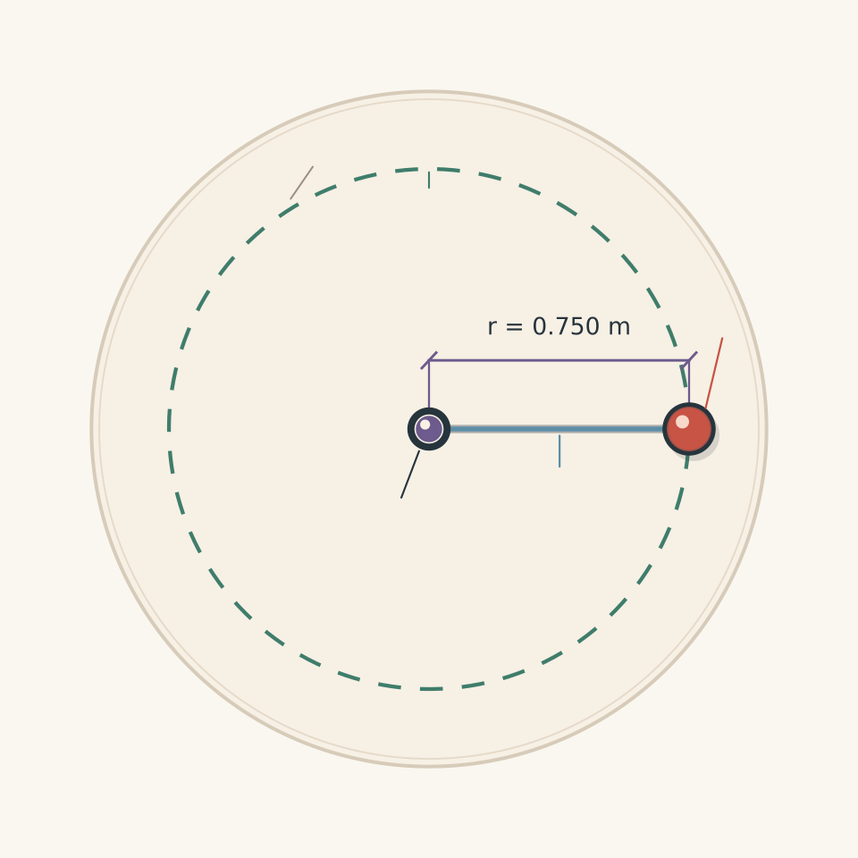
(a) Calculate the speed of the puck. (2 marks)
(b) Calculate the magnitude of its centripetal acceleration and state its direction. (2 marks)
(c) Calculate the magnitude of the net centripetal force acting on the puck. (2 marks)
(d) Identify the real force responsible for providing the centripetal force. Explain why the puck experiences acceleration even though its speed is constant. (2 marks)
Question 2 (10 marks)
A student investigates the relationship between centripetal force and speed using the rotating apparatus described in the exam instructions.
The mass and radius are kept constant:
- Mass: \(m = 0.200\text{ kg}\)
- Radius: \(r = 0.400\text{ m}\)
The student changes the rotational speed and records the force sensor reading.
The experimental results are shown below.
| Speed, \(v\) (m s⁻¹) | Measured force, \(F_c\) (N) | \(v^2\) (m² s⁻²) |
|---|---|---|
| 1.0 | 0.52 | |
| 1.5 | 1.10 | |
| 2.0 | 2.03 | |
| 2.5 | 3.08 | |
| 3.0 | 4.55 |
(a) Complete the final column by calculating \(v^2\) for each trial. (2 marks)
(b) State which variables should be plotted on the horizontal and vertical axes to produce a linear graph that tests the relationship between centripetal force and speed. Explain why your choice is appropriate. (2 marks)
(c) Plot the experimental data on graph paper. Include:
- Correctly labelled axes and units.
- An appropriate scale.
- All five experimental points.
- A straight line of best fit.
(2 marks)
(d) Use two widely separated points on your line of best fit to calculate its gradient. Include the appropriate units. (2 marks)
(e) Calculate the theoretical gradient predicted by the centripetal force model. Compare it with your experimental gradient and comment on whether the results support the model. (2 marks)
Question 3 (10 marks)
A student investigates how centripetal force changes with radius.
The experiment uses the same rotating apparatus as Question 2. This time, the mass and speed are kept constant while the radius is changed.
The experimental conditions are:
- Mass: \(m = 0.250\text{ kg}\)
- Speed: \(v = 3.00\text{ m s}^{-1}\)
The student records the following measurements.
| Radius, \(r\) (m) | Measured force, \(F_c\) (N) | \(1/r\) (m⁻¹) |
|---|---|---|
| 0.30 | 7.55 | |
| 0.40 | 5.72 | |
| 0.50 | 4.56 | |
| 0.60 | 3.78 | |
| 0.75 | 3.05 |
(a) Calculate \(1/r\) for each trial and complete the final column. (2 marks)
(b) State which variables should be plotted to produce a linear graph if the experimental results support the theoretical relationship. Explain your choice. (2 marks)
(c) Use two widely separated experimental points to estimate the gradient of the linearised relationship. Include the appropriate units. (2 marks)
(d) Calculate the theoretical gradient predicted by the centripetal force model. Compare this value with your experimental result. (2 marks)
(e) Explain how the student could ensure that speed remains constant while changing the radius. Explain why controlling speed is important when investigating the effect of radius on centripetal force. (2 marks)
Question 4 (10 marks)
A student investigates the relationship between centripetal force and mass.
Using the same rotating apparatus, the student varies the mass attached to the radial force sensor while maintaining a constant speed and radius.
The experimental conditions are:
- Speed: \(v = 2.40\text{ m s}^{-1}\)
- Radius: \(r = 0.600\text{ m}\)
The following results are recorded.
| Mass, \(m\) (kg) | Measured force, \(F_c\) (N) |
|---|---|
| 0.10 | 0.98 |
| 0.15 | 1.47 |
| 0.20 | 1.96 |
| 0.25 | 2.48 |
| 0.30 | 2.93 |
(a) Identify the variables that should be plotted to produce a linear graph. Explain why this graph is suitable for investigating the relationship between mass and centripetal force. (2 marks)
(b) Calculate the experimental gradient using the first and last data points. Include the appropriate units. (2 marks)
(c) Calculate the theoretical gradient predicted by the centripetal force model. (2 marks)
(d) Calculate the theoretical centripetal force for the \(0.250\text{ kg}\) mass. Compare your result with the experimental measurement. (2 marks)
(e) State the relationship between mass and centripetal force supported by these results. Identify the two variables that must remain constant to investigate this relationship fairly. (2 marks)
Question 5 (12 marks)
A student conducts an investigation to examine whether the speed of a rotating mass remains constant when the radius of its circular path changes.
The student uses a mass of \(0.250\text{ kg}\) and aims to maintain a speed of approximately \(3.0\text{ m s}^{-1}\).
For each radius, the student measures the time taken for ten complete revolutions and records the force sensor reading.
The results are shown below.
| Radius, \(r\) (m) | Time for 10 revolutions (s) | Measured force, \(F_c\) (N) |
|---|---|---|
| 0.30 | 6.3 | 7.6 |
| 0.40 | 8.4 | 5.7 |
| 0.50 | 10.4 | 4.6 |
| 0.60 | 13.0 | 3.6 |
The measurement uncertainties are:
- Radius: \(\pm 0.005\text{ m}\)
- Time for 10 revolutions: \(\pm 0.2\text{ s}\)
- Force sensor: \(\pm 0.1\text{ N}\)
(a) (2 marks) For the trial with a radius of \(0.400\text{ m}\), calculate:
i. The period of rotation.
ii. The speed of the rotating mass.
(b) Calculate the speeds for the trials with radii of \(0.300\text{ m}\) and \(0.600\text{ m}\).
Compare these results with the speed calculated in part (a). Describe any trend in the measurements. (3 marks)
(c) Using your calculated speed for the \(0.600\text{ m}\) trial, calculate the theoretical centripetal force.
Compare this result with the measured force and comment on their agreement. (2 marks)
(d) Calculate the maximum percentage uncertainty in the calculated speed for:
- The \(0.400\text{ m}\) trial.
- The \(0.600\text{ m}\) trial.
For this calculation, add the percentage uncertainties in radius and time.
Use your results to determine whether the two calculated speeds are consistent within their measurement uncertainties. (3 marks)
(e) Explain why timing ten revolutions is preferable to timing a single revolution. Suggest one further improvement that would increase the reliability or validity of this investigation. (2 marks)
03Worked solutions and marking guide
Solution 1
(a) Calculate the speed of the puck. (2 marks)
The speed of an object moving in uniform circular motion is the circumference of its circular path divided by the period.
\[ v=\frac{2\pi r}{T} \]
Substitute the given values:
\[ v=\frac{2\pi(0.750)}{1.50} \]
\[ \boxed{v=3.14\text{ m s}^{-1}} \]
Marking:
- Correct equation and substitution: 1 mark.
- Correct answer with units: 1 mark.
(b) Calculate centripetal acceleration and state its direction. (2 marks)
Centripetal acceleration is calculated using:
\[ a_c=\frac{v^2}{r} \]
Substitute the speed and radius:
\[ a_c=\frac{(3.1416)^2}{0.750} \]
\[ \boxed{a_c=13.2\text{ m s}^{-2}} \]
The acceleration points radially inwards, towards the centre of the circular path.
This direction is important. An object moving in a circle constantly changes the direction of its velocity, even if its speed remains unchanged.
Marking:
- Correct calculation: 1 mark.
- Correct inward direction: 1 mark.
(c) Calculate the centripetal force. (2 marks)
Centripetal force is the net inward force required to maintain circular motion.
\[ F_c=ma_c \]
Substitute:
\[ F_c=0.300(13.159) \]
\[ \boxed{F_c=3.95\text{ N}} \]
Marking:
- Correct equation and substitution: 1 mark.
- Correct answer with units: 1 mark.
(d) Identify the real force and explain why acceleration occurs. (2 marks)
The tension in the string provides the centripetal force.
The puck experiences acceleration because its velocity is constantly changing direction. Acceleration describes a change in velocity, not simply a change in speed.
Even though the puck travels at constant speed, its velocity is not constant. Therefore, it must accelerate towards the centre of the circle.
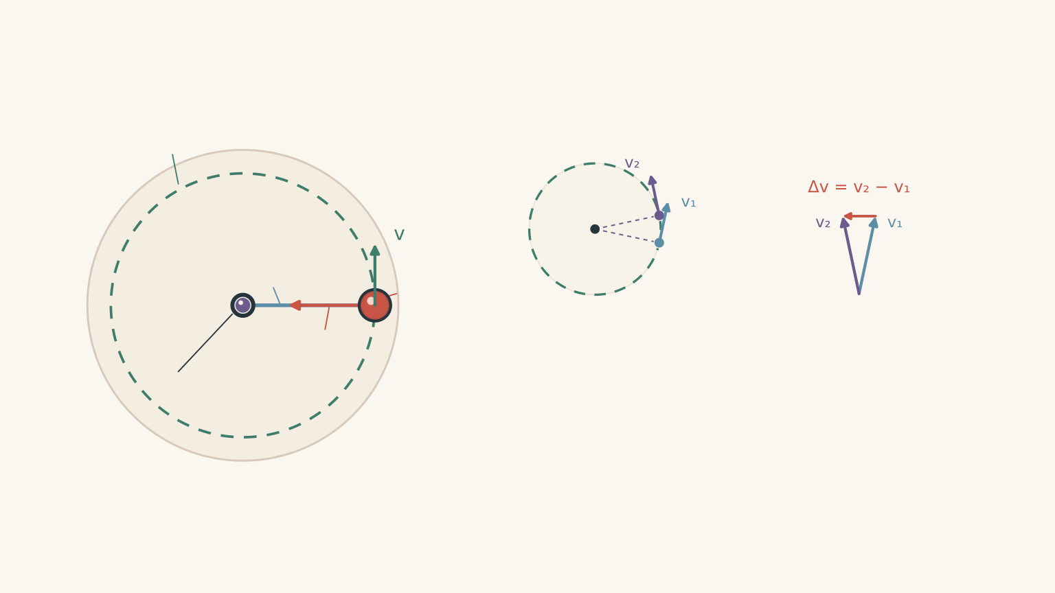
Marking:
- Identifies tension as the real force supplying the centripetal force: 1 mark.
- Explains that changing velocity direction produces acceleration: 1 mark.
Solution 2
(a) Complete the \(v^2\) column. (2 marks)
Square each measured speed.
For example:
\[ v^2=(1.5)^2=2.25\text{ m}^2\text{ s}^{-2} \]
The completed table is:
| Speed, \(v\) (m s⁻¹) | Force, \(F_c\) (N) | \(v^2\) (m² s⁻²) |
|---|---|---|
| 1.0 | 0.52 | 1.00 |
| 1.5 | 1.10 | 2.25 |
| 2.0 | 2.03 | 4.00 |
| 2.5 | 3.08 | 6.25 |
| 3.0 | 4.55 | 9.00 |
Marking:
- All five squared values correct: 2 marks.
- Minor calculation errors: 1 mark.
(b) Select the appropriate graph. (2 marks)
The horizontal axis should represent \(v^2\), while the vertical axis should represent \(F_c\).
This is because the centripetal force equation is:
\[ F_c=\frac{mv^2}{r} \]
Rearranging:
\[ F_c=\left(\frac{m}{r}\right)v^2 \]
The mass and radius are constant, so \(m/r\) is constant.
This means that a graph of \(F_c\) against \(v^2\) should produce a straight line.
Marking:
- Correctly identifies both axes: 1 mark.
- Explains why the relationship becomes linear: 1 mark.
(c) Plot the experimental data. (2 marks)
Your graph should have:
- Horizontal axis: \(v^2\), measured in \(\text{m}^2\text{ s}^{-2}\).
- Vertical axis: \(F_c\), measured in N.
- All five experimental points correctly plotted.
- A straight line of best fit passing close to the origin.
The graph should show that force increases as the square of speed increases.
Marking:
- Correct axes, units, and suitable scale: 1 mark.
- Correctly plotted points and appropriate line of best fit: 1 mark.
(d) Calculate the experimental gradient. (2 marks)
The gradient of a straight-line graph is:
\[ \text{Gradient}=\frac{\Delta y}{\Delta x} \]
For this graph:
\[ \text{Gradient}=\frac{\Delta F_c}{\Delta(v^2)} \]
Using the first and last experimental points:
\[ \text{Gradient} =\frac{4.55-0.52}{9.00-1.00} \]
\[ =\frac{4.03}{8.00} \]
\[ \boxed{\text{Gradient}=0.504\text{ kg m}^{-1}} \]
The gradient has units of \(\text{kg m}^{-1}\), as expected from dividing force by squared speed.
Small differences are acceptable when estimating the gradient from a drawn line of best fit.
Marking:
- Correct gradient calculation: 1 mark.
- Correct numerical value and units: 1 mark.
(e) Compare the experimental and theoretical gradients. (2 marks)
From the centripetal force equation:
\[ F_c=\frac{mv^2}{r} \]
The theoretical gradient of a graph of \(F_c\) against \(v^2\) is:
\[ \text{Gradient}=\frac{m}{r} \]
Substitute:
\[ \text{Gradient}=\frac{0.200}{0.400} \]
\[ \boxed{\text{Theoretical gradient}=0.500\text{ kg m}^{-1}} \]
Compare the values:
- Experimental gradient: \(0.504\text{ kg m}^{-1}\)
- Theoretical gradient: \(0.500\text{ kg m}^{-1}\)
The experimental value is very close to the theoretical value.
The difference is approximately \(0.8\%\), indicating strong agreement between the experimental results and the theoretical model.
The data therefore support the relationship:
\[ \boxed{F_c\propto v^2} \]
This conclusion applies while mass and radius remain constant.
Marking:
- Correct theoretical gradient: 1 mark.
- Comparison and appropriate conclusion: 1 mark.
Solution 3
(a) Calculate the reciprocal of each radius. (2 marks)
Calculate \(1/r\) for each experimental radius.
For example:
\[ \frac{1}{r}=\frac{1}{0.30} =3.33\text{ m}^{-1} \]
The completed table is:
| Radius, \(r\) (m) | Force, \(F_c\) (N) | \(1/r\) (m⁻¹) |
|---|---|---|
| 0.30 | 7.55 | 3.33 |
| 0.40 | 5.72 | 2.50 |
| 0.50 | 4.56 | 2.00 |
| 0.60 | 3.78 | 1.67 |
| 0.75 | 3.05 | 1.33 |
Marking:
- Correct reciprocal values: 2 marks.
- Minor rounding errors: 1 mark.
(b) Select the appropriate graph. (2 marks)
The horizontal axis should represent \(1/r\), while the vertical axis should represent \(F_c\).
Starting with:
\[ F_c=\frac{mv^2}{r} \]
Rearrange:
\[ F_c=mv^2\left(\frac{1}{r}\right) \]
Since mass and speed are constant, \(mv^2\) is constant.
Therefore, plotting \(F_c\) against \(1/r\) should produce a straight line.
This is an example of linearising an inverse relationship.
Marking:
- Correct choice of axes: 1 mark.
- Explanation of why the graph is linear: 1 mark.
(c) Calculate the experimental gradient. (2 marks)
The gradient is:
\[ \text{Gradient}= \frac{\Delta F_c}{\Delta(1/r)} \]
Using the first and last data points:
\[ \text{Gradient} =\frac{7.55-3.05}{3.33-1.33} \]
\[ =\frac{4.50}{2.00} \]
\[ \boxed{\text{Gradient}=2.25\text{ N m}} \]
The units are N m because the vertical axis is measured in newtons and the horizontal axis is measured in inverse metres.
Marking:
- Correct gradient calculation: 1 mark.
- Correct answer and units: 1 mark.
(d) Calculate and compare the theoretical gradient. (2 marks)
The theoretical gradient is:
\[ \text{Gradient}=mv^2 \]
Substitute:
\[ =0.250(3.00)^2 \]
\[ =0.250(9.00) \]
\[ \boxed{\text{Theoretical gradient}=2.25\text{ N m}} \]
Compare the results:
| Gradient | Value |
|---|---|
| Experimental | 2.25 N m |
| Theoretical | 2.25 N m |
The experimental gradient agrees with the theoretical prediction.
This provides strong evidence that centripetal force is inversely proportional to radius when mass and speed remain constant.
Marking:
- Correct theoretical calculation: 1 mark.
- Comparison with experimental result: 1 mark.
(e) Explain how to control speed. (2 marks)
The student must adjust the rotational rate as the radius changes to maintain a constant linear speed of \(3.00\text{ m s}^{-1}\).
One way to do this is to measure the period at each radius and calculate the speed using:
\[ v=\frac{2\pi r}{T} \]
The student can then adjust the rotation rate until the calculated speed matches the target.
Controlling speed is essential because:
\[ F_c=\frac{mv^2}{r} \]
Force depends on the square of speed. If speed changes during the experiment, changes in force cannot be attributed to radius alone.
Marking:
- Describes a suitable method for maintaining constant speed: 1 mark.
- Explains why changing speed would affect the investigation: 1 mark.
Solution 4
(a) Identify the appropriate graph. (2 marks)
Plot mass, \(m\), on the horizontal axis and centripetal force, \(F_c\), on the vertical axis.
The centripetal force equation is:
\[ F_c=\frac{mv^2}{r} \]
Rearranging:
\[ F_c=\left(\frac{v^2}{r}\right)m \]
Since speed and radius are constant, \(v^2/r\) is constant.
Therefore, force should be directly proportional to mass, producing a straight-line graph.
Marking:
- Correct axes: 1 mark.
- Explanation of the linear relationship: 1 mark.
(b) Calculate the experimental gradient. (2 marks)
Use the first and last data points:
\[ \text{Gradient}=\frac{\Delta F_c}{\Delta m} \]
\[ =\frac{2.93-0.98}{0.30-0.10} \]
\[ =\frac{1.95}{0.20} \]
\[ \boxed{\text{Gradient}=9.75\text{ N kg}^{-1}} \]
Marking:
- Correct gradient calculation: 1 mark.
- Correct value and units: 1 mark.
(c) Calculate the theoretical gradient. (2 marks)
The theoretical gradient is:
\[ \text{Gradient}=\frac{v^2}{r} \]
Substitute:
\[ =\frac{(2.40)^2}{0.600} \]
\[ =\frac{5.76}{0.600} \]
\[ \boxed{\text{Theoretical gradient}=9.60\text{ N kg}^{-1}} \]
Marking:
- Correct equation and substitution: 1 mark.
- Correct answer and units: 1 mark.
(d) Calculate the theoretical force for the 0.250 kg mass. (2 marks)
Use:
\[ F_c=\frac{mv^2}{r} \]
Substitute:
\[ F_c=\frac{0.250(2.40)^2}{0.600} \]
\[ F_c=\frac{0.250(5.76)}{0.600} \]
\[ \boxed{F_c=2.40\text{ N}} \]
The experimental measurement was \(2.48\text{ N}\).
The difference is:
\[ 2.48-2.40=0.08\text{ N} \]
The measured force is slightly higher than the theoretical prediction, but the two values are close.
The results are broadly consistent with the theoretical model. The absence of a stated measurement uncertainty means we cannot make a more definite claim about the significance of this difference.
Marking:
- Correct theoretical force: 1 mark.
- Comparison with the experimental value: 1 mark.
(e) State the relationship and identify the control variables. (2 marks)
The experimental data support a directly proportional relationship between mass and centripetal force.
In other words:
\[ \boxed{F_c\propto m} \]
This relationship applies when speed and radius remain constant.
The two control variables are:
- Speed of the rotating mass.
- Radius of the circular path.
If either changes, it affects the centripetal force and makes it harder to isolate the effect of mass.
Marking:
- Identifies the direct proportional relationship: 1 mark.
- Correctly identifies speed and radius as control variables: 1 mark.
Solution 5
(a) Calculate the period and speed for the 0.400 m trial. (2 marks)
First, calculate the period.
The student measures ten revolutions in \(8.4\text{ s}\).
Therefore:
\[ T=\frac{8.4}{10} \]
\[ \boxed{T=0.840\text{ s}} \]
Now calculate the speed:
\[ v=\frac{2\pi r}{T} \]
Substitute:
\[ v=\frac{2\pi(0.400)}{0.840} \]
\[ \boxed{v=2.99\text{ m s}^{-1}} \]
Marking:
- Correct period: 1 mark.
- Correct speed and units: 1 mark.
(b) Calculate and compare the speeds. (3 marks)
For the \(0.300\text{ m}\) trial:
The period is:
\[ T=\frac{6.3}{10}=0.630\text{ s} \]
Calculate the speed:
\[ v=\frac{2\pi(0.300)}{0.630} \]
\[ \boxed{v=2.99\text{ m s}^{-1}} \]
For the \(0.600\text{ m}\) trial:
The period is:
\[ T=\frac{13.0}{10}=1.30\text{ s} \]
Calculate the speed:
\[ v=\frac{2\pi(0.600)}{1.30} \]
\[ \boxed{v=2.90\text{ m s}^{-1}} \]
Compare the results:
| Radius (m) | Calculated speed (m s⁻¹) |
|---|---|
| 0.300 | 2.99 |
| 0.400 | 2.99 |
| 0.600 | 2.90 |
The calculated speeds are relatively similar.
However, the \(0.600\text{ m}\) trial has a slightly lower calculated speed. The difference between the \(0.400\text{ m}\) and \(0.600\text{ m}\) trials is approximately \(3.0\%\).
This suggests that the student has maintained approximately constant speed, although the central measured values are not identical.
Marking:
- Correct speed for the \(0.300\text{ m}\) trial: 1 mark.
- Correct speed for the \(0.600\text{ m}\) trial: 1 mark.
- Appropriate comparison and interpretation: 1 mark.
(c) Calculate and compare the centripetal force. (2 marks)
For the \(0.600\text{ m}\) trial, use the calculated speed of \(2.90\text{ m s}^{-1}\).
The theoretical centripetal force is:
\[ F_c=\frac{mv^2}{r} \]
Substitute:
\[ F_c=\frac{0.250(2.90)^2}{0.600} \]
\[ =\frac{0.250(8.41)}{0.600} \]
\[ \boxed{F_c=3.50\text{ N}} \]
The measured force is \(3.6\text{ N}\).
The difference is:
\[ 3.6-3.50=0.10\text{ N} \]
The difference equals the stated force sensor uncertainty of \(\pm0.1\text{ N}\).
The experimental and theoretical values are therefore compatible at the stated measurement precision.
Marking:
- Correct theoretical force calculation: 1 mark.
- Comparison with the experimental reading: 1 mark.
(d) Calculate the maximum percentage uncertainties. (3 marks)
The speed equation is:
\[ v=\frac{2\pi r}{T} \]
For a quotient, the maximum percentage uncertainty is estimated by adding the percentage uncertainties in the numerator and denominator.
Therefore:
\[ \%\Delta v= \frac{\Delta r}{r}\times100 + \frac{\Delta T}{T}\times100 \]
Remember that the uncertainty in the period is the uncertainty in the total time divided by ten.
For the \(0.400\text{ m}\) trial:
Radius uncertainty:
\[ \frac{0.005}{0.400}\times100=1.25\% \]
Time uncertainty:
\[ \frac{0.2}{8.4}\times100=2.38\% \]
Total maximum percentage uncertainty:
\[ 1.25+2.38=3.63\% \]
\[ \boxed{\%\Delta v=3.63\%} \]
For the \(0.600\text{ m}\) trial:
Radius uncertainty:
\[ \frac{0.005}{0.600}\times100=0.833\% \]
Time uncertainty:
\[ \frac{0.2}{13.0}\times100=1.54\% \]
Total maximum percentage uncertainty:
\[ 0.833+1.54=2.37\% \]
\[ \boxed{\%\Delta v=2.37\%} \]
Now consider the uncertainty intervals for the two calculated speeds.
For the \(0.400\text{ m}\) trial:
\[ v=2.99\pm3.63\% \]
This gives an approximate range of:
\[ 2.88\text{ to }3.10\text{ m s}^{-1} \]
For the \(0.600\text{ m}\) trial:
\[ v=2.90\pm2.37\% \]
This gives an approximate range of:
\[ 2.83\text{ to }2.97\text{ m s}^{-1} \]
The two ranges overlap.
Therefore, despite the difference in their calculated central values, the speeds are consistent within the estimated measurement uncertainties.
The data do not provide sufficient evidence to conclude that the speed changed significantly between these two trials.
Marking:
- Correct maximum percentage uncertainty for the \(0.400\text{ m}\) trial: 1 mark.
- Correct maximum percentage uncertainty for the \(0.600\text{ m}\) trial: 1 mark.
- Correctly interprets the overlapping uncertainty ranges: 1 mark.
(e) Explain the timing method and suggest an improvement. (2 marks)
Timing ten revolutions instead of one reduces the relative effect of stopwatch reaction time.
For example, an uncertainty of \(0.2\text{ s}\) represents a much smaller percentage of a total time of \(8.4\text{ s}\) than it would of a single revolution lasting \(0.84\text{ s}\).
This makes the calculated period more reliable.
One further improvement would be to use an electronic revolution counter or photogate. This reduces uncertainty associated with manually starting and stopping a stopwatch.
Other acceptable improvements include:
- Repeating each trial several times and calculating an average.
- Measuring the radius carefully from the axis of rotation to the centre of the mass.
- Using a speed-monitoring system to maintain a consistent linear speed throughout the experiment.
Marking:
- Explains how timing multiple revolutions reduces relative timing uncertainty: 1 mark.
- Provides one appropriate experimental improvement: 1 mark.
For further practice on this syllabus scope, try the tutorgum Circular Motion Investigations: Physics Practice Exam.