
How to Choose Graph Axes and Linearise HSC Physics Data
Learn how to choose independent and dependent variables, label graph axes correctly, and transform HSC Physics data into straight-line relationships. Use worked examples from motion, electrical circuits, and inverse-square light intensity to interpret gradients, intercepts, and common graphing mistakes.
You put time on the vertical axis, displacement on the horizontal axis, draw a perfectly neat straight line, and report its gradient as velocity. The units quietly give you away: your gradient is in seconds per metre, not metres per second. Or you see a curved displacement-time graph and plot displacement against time squared, expecting a straight line simply because the object accelerates. The graph still curves.
These are not drawing mistakes. They are mistakes in choosing variables and interpreting the physical model. Fix those decisions before you pick up a ruler.
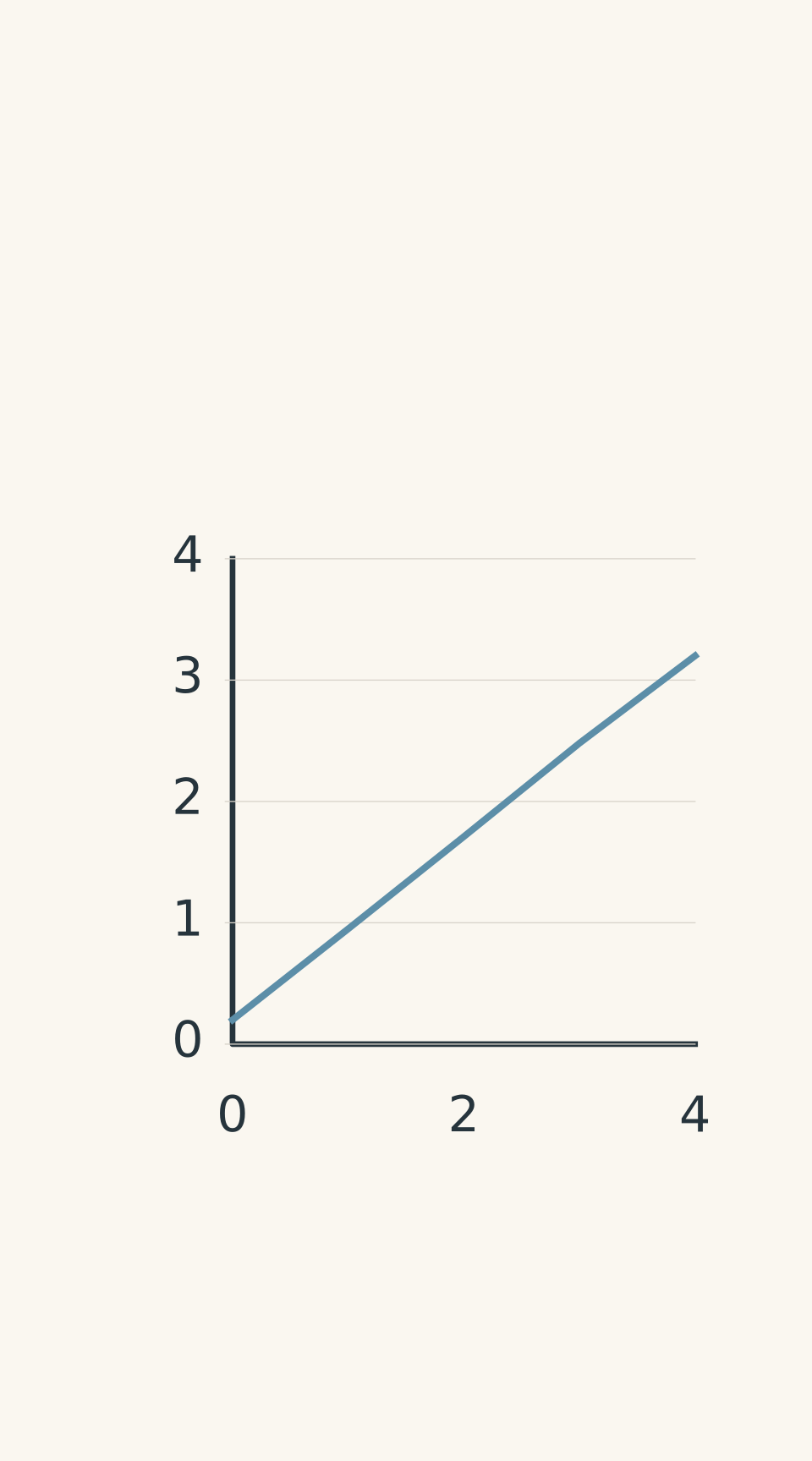
- Trolley measurements; best-fit gradient ≈ 0.75 m/s
01Choose the axes before drawing the graph
The first decision is simple: what are you changing, and what are you measuring in response?
The independent variable is the variable you deliberately change, or the variable you use to explain a pattern in the data. It normally belongs on the horizontal axis.
The dependent variable is the quantity you measure in response. It normally belongs on the vertical axis.
For example, if you measure a trolley’s displacement at different times, time is the independent variable and displacement is the dependent variable. You plot displacement vertically against time horizontally.
There is also a useful translation rule for exam questions:
“Plot A against B” means A goes on the vertical axis and B goes on the horizontal axis.
So:
- Plot voltage against current: voltage vertically, current horizontally.
- Plot velocity against time: velocity vertically, time horizontally.
- Plot illuminance against reciprocal distance squared: illuminance vertically, \(1/r^2\) horizontally.
The order in which quantities appear in a data table does not determine the axes. Neither does whichever arrangement happens to produce a straighter line.
Label both axes properly
Every axis needs the quantity, its symbol, and its unit.
| Quantity | Suitable axis label |
|---|---|
| Time | Time, \(t\) (s) |
| Displacement | Displacement, \(x\) (m) |
| Velocity | Velocity, \(v\) (m/s) |
| Acceleration | Acceleration, \(a\) (m/s²) |
| Current | Current, \(I\) (A) |
| Voltage | Voltage, \(V\) (V) |
| Distance | Distance, \(r\) (m) |
| Illuminance | Illuminance, \(E\) (lx) |
Notice the difference between labelling an axis Time, t (s) and labelling it simply seconds. The first tells the reader what is being measured and which unit is used. The second gives only the unit.
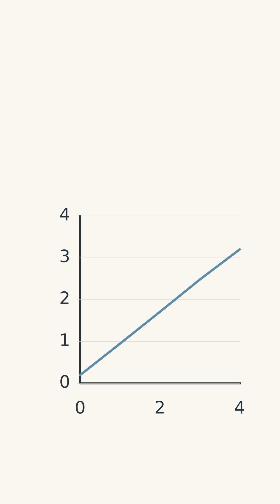
- Trolley measurements
Choose a sensible, evenly spaced scale that uses the available graph area. Experimental points should be plotted accurately, with a line of best fit where appropriate.
For continuous physics data, a scatter graph is usually the right starting point. Do not automatically join every point with straight segments. Your aim is to identify the relationship between the variables, not to create a connect-the-dots picture.
02Work out what relationship the graph should show
Before deciding whether to draw a straight line or a curve, write down the physical model.
This is where many otherwise sensible graphing methods go wrong. Students often see a curve and start trying transformations until the data look straight. A better approach is to predict the graph from the equation.
For the motion equations below, \(x\) is position in metres, \(x_0\) is initial position, \(t\) is time in seconds, \(v\) is velocity in metres per second, \(u\) is initial velocity, and \(a\) is acceleration in metres per second squared. Displacement from the initial position is \(\Delta x=x-x_0\).
For circuits, \(V\) is voltage in volts, \(I\) is current in amperes, and \(R\) is resistance in ohms. For light, \(E\) is illuminance in lux, \(E_{\mathrm{bg}}\) is background illuminance, \(r\) is distance in metres, and \(k\) is a proportionality constant.
Here are some relationships worth recognising.
| Physical relationship | Suitable graph | Meaning of gradient |
|---|---|---|
| \(x=x_0+vt\), for constant velocity | \(x\) against \(t\) | Velocity, \(v\) |
| \(v=u+at\), for constant acceleration | \(v\) against \(t\) | Acceleration, \(a\) |
| \(\Delta x=\frac12 at^2\), when \(u=0\) | \(\Delta x\) against \(t^2\) | Half the acceleration, \(a/2\) |
| \(V=RI\), for an ohmic resistor at constant temperature | \(V\) against \(I\) | Resistance, \(R\) |
| \(E=E_{\mathrm{bg}}+\frac{k}{r^2}\) | \(E\) against \(1/r^2\) | Constant, \(k\) |
The conditions matter. In particular, the third row assumes the object starts from rest and that displacement is measured from its starting position. Without those conditions, the proposed straight-line graph may not work.
- Trolley data; gradient ≈ 0.75 m/s
What does it mean to linearise data?
To linearise a relationship is to transform one or both plotted variables so that the model predicts a straight line.
A straight-line relationship can be written as
\[ Y=mX+c \]
where:
- \(Y\) is the vertical variable.
- \(X\) is the horizontal variable.
- \(m\) is the gradient.
- \(c\) is the vertical intercept.
The key is that \(X\) and \(Y\) can be transformed variables, rather than the original measurements.
For example, if a model predicts
\[ y=kx^2 \]
then plotting \(y\) against \(x\) produces a curve. Plotting \(y\) against \(x^2\) instead produces a straight line, because the model becomes \(y=kX\), where \(X=x^2\).
But be careful. If the original equation contains additional terms, such as \(y=bx+cx^2\), plotting \(y\) against \(x^2\) will not generally produce a straight line. The \(bx\) term is still present.
This is why you should derive a transformation from the physical model rather than guess one.
From physical model to meaningful graph
- Identify the variables
Independent: horizontal axis; dependent: vertical axis.
- Write the physical model
Identify the relationship and its assumptions.
- Choose the graph
Plot the original variables or derive a justified transformation.
- Interpret the line
Use the actual axes to determine gradient units, physical meaning, and intercept.
03Recognise the three relationships that commonly cause trouble
Motion: constant acceleration does not always mean displacement is proportional to time squared
For constant acceleration, displacement is described by
\[ \Delta x=ut+\frac12at^2 \]
If the object starts from rest, then \(u=0\), so
\[ \Delta x=\frac12at^2 \]
This simplified equation predicts a straight line when you plot \(\Delta x\) against \(t^2\). The gradient is \(a/2\), not \(a\).
If the object has a non-zero initial velocity, the \(ut\) term remains. Plotting displacement against time squared will generally produce a curve.
You have two options: use a velocity-time graph if velocity data are available, or find a transformation that accounts for the initial velocity. The second approach appears in Question 5.
Circuits: the gradient depends on which quantity is vertical
For an ohmic resistor at constant temperature,
\[ V=IR \]
If voltage is vertical and current is horizontal, the graph’s gradient is
\[ m=\frac{\Delta V}{\Delta I}=R \]
Its units are volts per ampere, equivalent to ohms.
Reverse the axes and you get a different gradient:
\[ m=\frac{\Delta I}{\Delta V}=\frac1R \]
That is conductance, not resistance.
Both graphs can be perfectly straight. Only one has a gradient equal to resistance.
Light intensity: inverse-square relationships need a transformed axis
For an ideal point source, with background illumination removed, illuminance follows an inverse-square relationship:
\[ E=\frac{k}{r^2} \]
Doubling the distance reduces the illuminance to one-quarter of its original value. Tripling the distance reduces it to one-ninth.
A graph of \(E\) against \(r\) is curved. A graph of \(E\) against \(1/r^2\) should be linear under the model’s assumptions.
The horizontal axis now has units of \(\mathrm{m^{-2}}\). The gradient has units of \(\mathrm{lx\,m^2}\), because it is illuminance divided by reciprocal distance squared.
If background light has not been removed, the more realistic model is
\[ E=E_{\mathrm{bg}}+\frac{k}{r^2} \]
The graph of \(E\) against \(1/r^2\) should still be straight, but its intercept is \(E_{\mathrm{bg}}\), rather than zero.
04Interpret the gradient and intercept correctly
Once you have chosen the axes, the mathematics is straightforward. The important part is interpreting the result.
The gradient
For a graph with vertical variable \(Y\) and horizontal variable \(X\),
\[ m=\frac{\Delta Y}{\Delta X} \]
Calculate the change in the vertical quantity divided by the change in the horizontal quantity.
Use two well-separated points on the line of best fit, rather than two nearby raw data points. This reduces the effect of small reading errors. The points you use to calculate the gradient do not have to be original measurements, provided they lie on the best-fit line.
Always check the units.
- Displacement against time: \(\mathrm{m/s}\).
- Velocity against time: \(\mathrm{m/s^2}\).
- Voltage against current: \(\mathrm{V/A}=\Omega\).
- Illuminance against \(1/r^2\): \(\mathrm{lx\,m^2}\).
If the units do not match the physical quantity you claim to have calculated, stop and check your axes.
Also, do not confuse the gradient with the ratio \(Y/X\). They are equal only for a straight line passing through the origin. If the intercept is non-zero, use changes in the quantities to calculate the gradient.
The intercept
The vertical intercept is the value of the vertical variable when the horizontal variable equals zero.
It might represent:
- Initial position on a displacement-time graph.
- Initial velocity on a velocity-time graph.
- Background illuminance on a graph of illuminance against \(1/r^2\).
- A measurement offset in an electrical experiment.
A non-zero intercept is not automatically an experimental mistake. It may be predicted by the model.
Likewise, do not force a best-fit line through the origin simply because the equation you remember has no constant term. First check whether the experimental conditions support that model and whether the measurements are consistent with it.
Same straight-line form, different physical meanings
| Displacement–time | x = x₀ + vt Horizontal: t (s); vertical: x (m). Gradient v (m/s); intercept x₀ (m), initial position. |
|---|---|
| Velocity–time | v = u + at Horizontal: t (s); vertical: v (m/s). Gradient a (m/s²); intercept u (m/s), initial velocity. |
| Inverse-square light | E = E_bg + k(1/r²) Horizontal: 1/r² (m⁻²); vertical: E (lx). Gradient k (lx·m²); intercept E_bg (lx), background illuminance. |
05Worked examples
Worked example: finding velocity from displacement-time data
A trolley’s displacement from a fixed origin is measured at several times.
| Time, \(t\) (s) | Displacement, \(x\) (m) |
|---|---|
| 0 | 0.20 |
| 1 | 0.95 |
| 2 | 1.71 |
| 3 | 2.48 |
| 4 | 3.20 |
Choose the axes, estimate the trolley’s velocity and initial position, and explain what would happen if the axes were reversed.
Step 1
Time is the independent variable, and displacement is the dependent variable.
Put time on the horizontal axis and displacement on the vertical axis. Label them Time, t (s) and Displacement, x (m).
Step 2
The points lie approximately on a straight line, which is consistent with constant velocity. Do not force the line through the origin; the initial displacement is not zero.
Step 3
Using the endpoints of the best-fit line as an estimate,
\[ \begin{aligned} v&=\frac{\Delta x}{\Delta t}\\ &=\frac{3.20-0.20}{4.0-0}\\ &=\frac{3.00\ \mathrm{m}}{4.0\ \mathrm{s}}\\ &=0.75\ \mathrm{m/s} \end{aligned} \]
The trolley’s velocity is approximately \(0.75\ \mathrm{m/s}\).
Step 4
The line crosses the vertical axis at approximately \(0.20\ \mathrm{m}\). This is the initial position \(x_0\).
The relationship is therefore approximately
\[ x=0.20+0.75t \]
where \(x\) is in metres and \(t\) is in seconds.
If you reversed the axes, the gradient would have units of \(\mathrm{s/m}\). It would describe the change in time per unit displacement, not velocity. A straight line does not guarantee that you have calculated the quantity you intended.
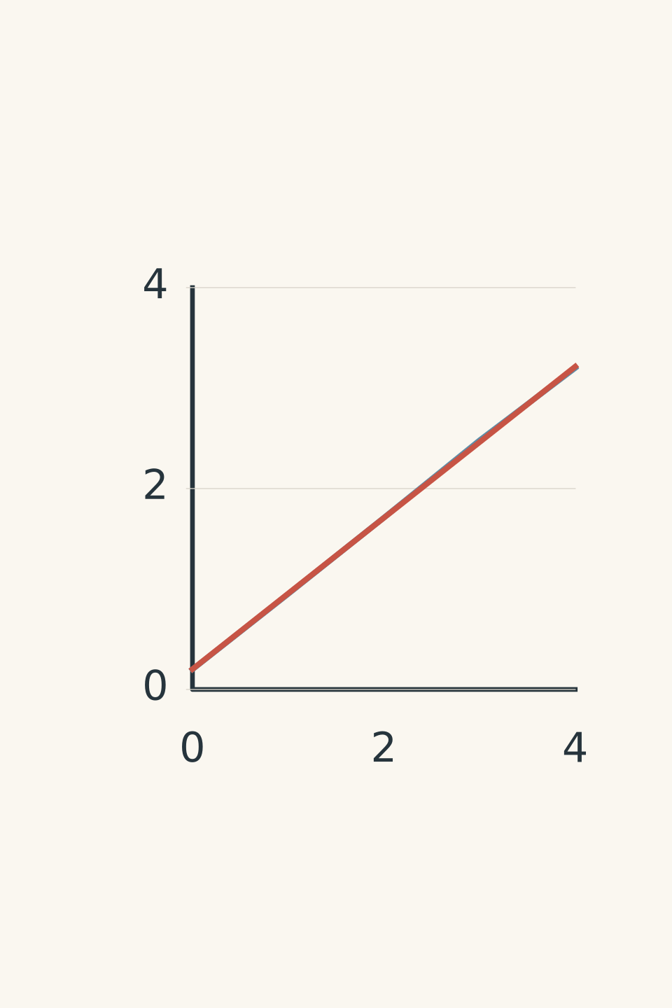
- Measured data
- Best fit, 0.75 m/s
Worked example: finding resistance from circuit measurements
A student measures the voltage across a resistor at different currents.
| Current, \(I\) (A) | Voltage, \(V\) (V) |
|---|---|
| 0.10 | 0.48 |
| 0.20 | 1.01 |
| 0.30 | 1.49 |
| 0.40 | 2.02 |
| 0.50 | 2.51 |
Estimate the resistance from the graph and comment on the intercept.
Step 1
Current is the independent variable, and voltage is the dependent variable. Plot \(V\) vertically against \(I\) horizontally.
Step 2
For an ohmic resistor at constant temperature,
\[ V=IR \]
Comparing this with \(Y=mX+c\), the gradient of a voltage-current graph is the resistance.
Step 3
Using the first and last measurements to estimate the gradient of the best-fit line,
\[ \begin{aligned} R&=\frac{\Delta V}{\Delta I}\\ &=\frac{2.51-0.48}{0.50-0.10}\\ &=\frac{2.03\ \mathrm{V}}{0.40\ \mathrm{A}}\\ &=5.075\ \Omega\\ &\approx 5.1\ \Omega \end{aligned} \]
The estimated resistance is \(5.1\ \Omega\).
Step 4
Using the estimated gradient and the first measurement,
\[ \begin{aligned} c&\approx V-RI\\ &=0.48-(5.075)(0.10)\\ &\approx -0.03\ \mathrm{V} \end{aligned} \]
This is close to zero compared with the measurement scatter. The data are consistent with the ideal model, although the small calculated intercept should not be overinterpreted.
The tempting mistake is to reverse the axes and still call the gradient resistance. If current is vertical and voltage is horizontal, the gradient represents \(1/R\). Always identify the vertical and horizontal quantities before interpreting the slope.
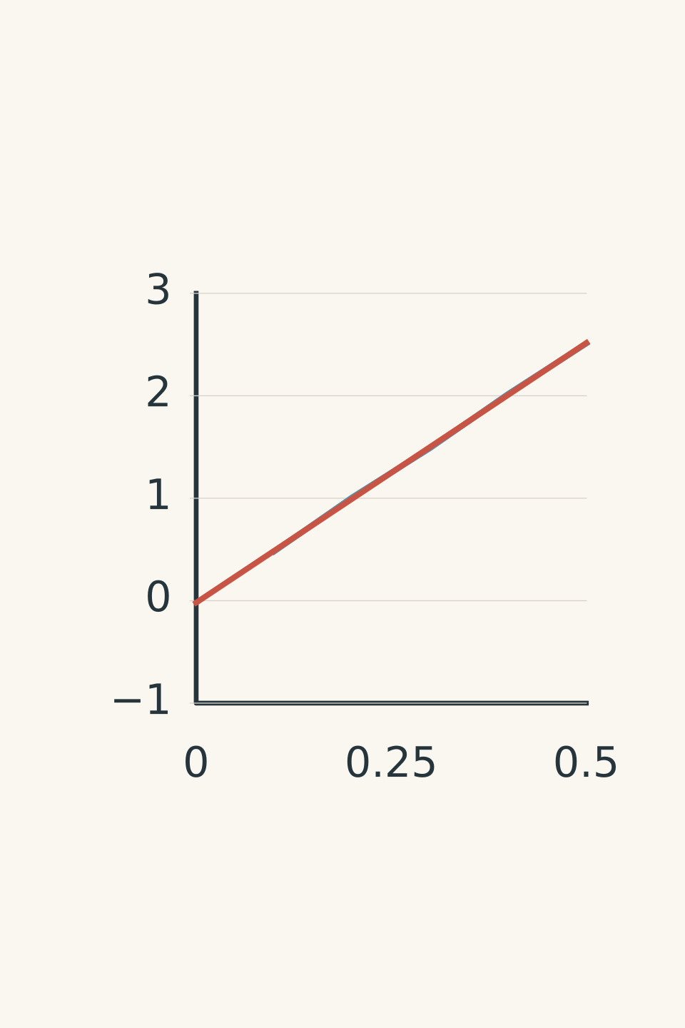
- Measured data
- Best fit: gradient ≈ 5.1 Ω
Worked example: linearising inverse-square light data
An idealised point-source experiment produces the following background-corrected illuminance measurements.
| Distance, \(r\) (m) | Illuminance, \(E\) (lx) |
|---|---|
| 0.50 | 40.0 |
| 0.70 | 20.4 |
| 1.00 | 10.0 |
| 1.40 | 5.1 |
| 2.00 | 2.5 |
Assume the source output and detector orientation remain constant. Choose a graph that tests the inverse-square model and estimate \(k\) in \(E=k/r^2\).
Step 1
Distance is the independent variable, and illuminance is the dependent variable.
A graph of \(E\) against \(r\) should be curved if the inverse-square model is correct. A curved graph does not, by itself, mean the model has failed.
Step 2
The model is
\[ E=\frac{k}{r^2} \]
Rewrite it as
\[ E=k\left(\frac1{r^2}\right) \]
Now plot \(E\) vertically against \(1/r^2\) horizontally.
Calculate the transformed values:
| \(1/r^2\) (m⁻²) | \(E\) (lx) |
|---|---|
| 4.00 | 40.0 |
| 2.04 | 20.4 |
| 1.00 | 10.0 |
| 0.510 | 5.1 |
| 0.250 | 2.5 |
Step 3
Using the points \((4.00,\ 40.0)\) and \((0.250,\ 2.5)\),
\[ \begin{aligned} k&=\frac{\Delta E}{\Delta(1/r^2)}\\ &=\frac{40.0-2.5}{4.00-0.250}\\ &=\frac{37.5\ \mathrm{lx}}{3.75\ \mathrm{m^{-2}}}\\ &=10.0\ \mathrm{lx\,m^2} \end{aligned} \]
The estimated constant is \(k=10.0\ \mathrm{lx\,m^2}\).
This means the model predicts \(E=10.0/r^2\), with \(r\) measured in metres. The gradient has the correct units because illuminance is divided by reciprocal distance squared.
The transformation is justified by the inverse-square model, not merely by the fact that the transformed graph looks straight.
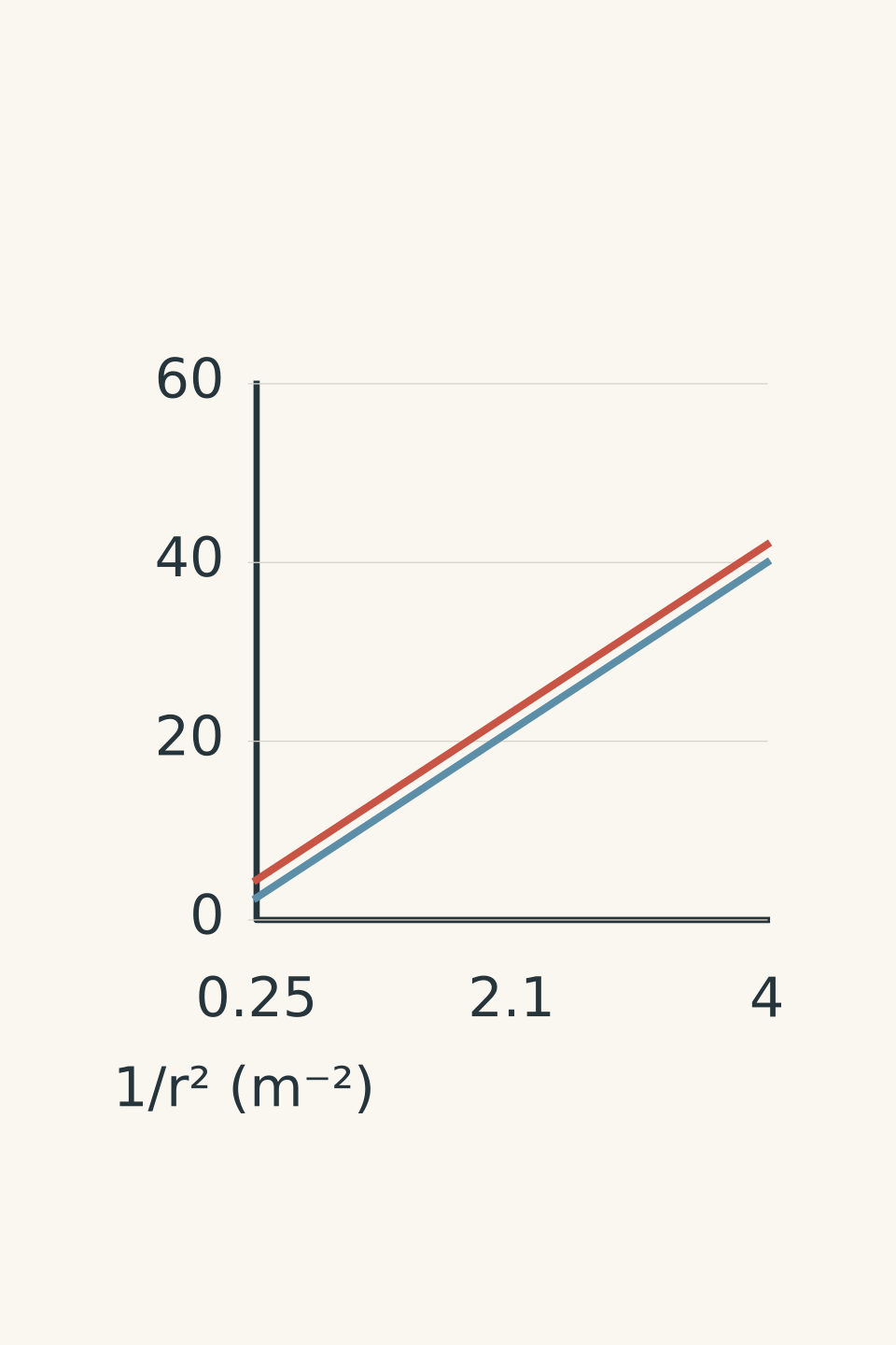
- Background corrected
- With 2 lx background (schematic)
06The 20-second exam check
Before submitting a graph, check these points:
- [ ] Have I identified the independent and dependent variables?
- [ ] Does “plot A against B” put A on the vertical axis and B on the horizontal axis?
- [ ] Does each axis show the quantity, symbol, and unit?
- [ ] If I transformed a variable, can I derive that transformation from the physical model?
- [ ] Are the units of my gradient consistent with the quantity I claim to have calculated?
- [ ] Have I interpreted the intercept using the actual conditions, rather than assuming it must be zero?
- [ ] Have I drawn a suitable best-fit line or curve instead of automatically joining every point?
07Questions and solutions
Question 1
A cyclist’s displacement is recorded as follows.
| Time, \(t\) (s) | Displacement, \(x\) (m) |
|---|---|
| 0 | 0.0 |
| 1 | 2.4 |
| 2 | 4.9 |
| 3 | 7.1 |
Choose the axes and estimate the cyclist’s average velocity. Explain why reversing the axes would change the meaning of the gradient.
Solution 1
Plot displacement \(x\) vertically against time \(t\) horizontally. The gradient gives an average velocity of approximately \(2.4\ \mathrm{m/s}\).
Using the first and last measurements,
\[ \begin{aligned} v_{\mathrm{avg}}&=\frac{\Delta x}{\Delta t}\\ &=\frac{7.1-0.0}{3.0-0}\\ &=\frac{7.1\ \mathrm{m}}{3.0\ \mathrm{s}}\\ &\approx 2.37\ \mathrm{m/s} \end{aligned} \]
A best-fit line through all four points gives a similar estimate.
If the axes were reversed, the gradient would have units of \(\mathrm{s/m}\). It would describe the change in time per unit displacement, not the cyclist’s velocity. The physical meaning of a gradient depends on the quantities actually plotted.
Question 2
An incandescent lamp produces the following measurements.
| Current, \(I\) (A) | Voltage, \(V\) (V) |
|---|---|
| 0.20 | 1.0 |
| 0.40 | 2.4 |
| 0.60 | 4.2 |
A student argues that the voltage-current graph must be a straight line because \(V=IR\). They also calculate the gradient between the first and last points and claim that it is the lamp’s resistance at every current.
Calculate \(V/I\) at each measurement, find the gradient between the first and last points, and explain both errors. Would plotting \(V\) against \(I^2\) automatically linearise the data?
Solution 2
The lamp’s resistance increases across these measurements, and the gradient between the first and last points is not its resistance at every operating current. The equation \(V=IR\) predicts a straight line only when \(R\) remains constant.
Calculate the voltage-to-current ratio at each point:
\[ \begin{aligned} R_1&=\frac{1.0}{0.20}=5.0\ \Omega\\ R_2&=\frac{2.4}{0.40}=6.0\ \Omega\\ R_3&=\frac{4.2}{0.60}=7.0\ \Omega \end{aligned} \]
The ratio \(V/I\) increases from \(5.0\ \Omega\) to \(7.0\ \Omega\).
Now calculate the gradient between the first and last points:
\[ \begin{aligned} m&=\frac{\Delta V}{\Delta I}\\ &=\frac{4.2-1.0}{0.60-0.20}\\ &=\frac{3.2\ \mathrm{V}}{0.40\ \mathrm{A}}\\ &=8.0\ \Omega \end{aligned} \]
This is the average change in voltage per change in current over that interval. It is not the value of \(V/I\) at every point. For a curved voltage-current graph, the gradient of a tangent at a particular point describes the local rate of change of voltage with current, which need not equal \(V/I\).
The physical reason for the curvature is that the filament heats up as current increases. Its temperature changes, so its resistance is not constant. The usual straight-line prediction for an ohmic resistor assumes constant temperature.
Finally, plotting \(V\) against \(I^2\) is not automatically justified. The data show that \(V/I\) increases, but they do not establish a model in which voltage is proportional to current squared. A transformation should follow from a justified physical relationship, not from a guess about which graph might look straight.
Question 3
A student measures illuminance at three distances from a light source.
| Distance, \(r\) (m) | Illuminance, \(E\) (lx) |
|---|---|
| 0.50 | 50 |
| 1.00 | 14 |
| 2.00 | 5 |
The measurements include a constant background illuminance. Assume the model
\[ E=E_{\mathrm{bg}}+\frac{k}{r^2} \]
where \(E_{\mathrm{bg}}\) is the background illuminance and \(k\) is a constant.
Choose the correct graph, determine \(k\) and \(E_{\mathrm{bg}}\), and explain why forcing the graph through the origin would be inappropriate.
Solution 3
Plot illuminance \(E\) vertically against reciprocal distance squared \(1/r^2\) horizontally. The gradient is \(k=12\ \mathrm{lx\,m^2}\), and the vertical intercept is \(E_{\mathrm{bg}}=2\ \mathrm{lx}\).
First, transform the distances:
| \(r\) (m) | \(1/r^2\) (m⁻²) | \(E\) (lx) |
|---|---|---|
| 0.50 | 4.00 | 50 |
| 1.00 | 1.00 | 14 |
| 2.00 | 0.25 | 5 |
Using the first two points, the gradient is
\[ \begin{aligned} k&=\frac{50-14}{4.00-1.00}\\ &=\frac{36\ \mathrm{lx}}{3.00\ \mathrm{m^{-2}}}\\ &=12\ \mathrm{lx\,m^2} \end{aligned} \]
Check the remaining interval:
\[ \frac{14-5}{1.00-0.25} =\frac{9}{0.75} =12\ \mathrm{lx\,m^2} \]
The data are consistent with a straight line.
At \(r=1.00\ \mathrm{m}\), the reciprocal-square value is \(1.00\ \mathrm{m^{-2}}\). Therefore,
\[ \begin{aligned} E_{\mathrm{bg}}&=E-\frac{k}{r^2}\\ &=14-12(1.00)\\ &=2\ \mathrm{lx} \end{aligned} \]
The model is consequently
\[ E=2+\frac{12}{r^2} \]
The tempting mistake is to assume that inverse-square behaviour requires a line through the origin. It requires a straight line when \(E\) is plotted against \(1/r^2\), but the background light adds a constant to every reading. Forcing the line through the origin would hide this contribution and distort the estimated gradient.
Question 4
A cart’s velocity is recorded over four seconds.
| Time, \(t\) (s) | Velocity, \(v\) (m/s) |
|---|---|
| 0 | 6 |
| 1 | 3 |
| 2 | 0 |
| 3 | −3 |
| 4 | −6 |
Plot velocity against time. Determine the cart’s acceleration, displacement over the four seconds, and total distance travelled.
A student claims that the gradient gives displacement and the area under the graph always gives distance. Explain why both claims are incorrect.
Solution 4
The cart’s acceleration is \(-3.0\ \mathrm{m/s^2}\), its displacement is \(0\ \mathrm{m}\), and its total distance travelled is \(12\ \mathrm{m}\).
Plot velocity \(v\) vertically against time \(t\) horizontally.
The gradient gives acceleration:
\[ \begin{aligned} a&=\frac{\Delta v}{\Delta t}\\ &=\frac{-6-6}{4-0}\\ &=\frac{-12\ \mathrm{m/s}}{4\ \mathrm{s}}\\ &=-3.0\ \mathrm{m/s^2} \end{aligned} \]
The negative gradient means the velocity decreases with time.
To find displacement, calculate the signed area under the velocity-time graph. From \(t=0\) to \(t=2\ \mathrm{s}\), the positive triangular area is
\[ A_+=\frac12(2\ \mathrm{s})(6\ \mathrm{m/s})=6\ \mathrm{m} \]
From \(t=2\) to \(t=4\ \mathrm{s}\), the negative triangular area is
\[ A_-=-\frac12(2\ \mathrm{s})(6\ \mathrm{m/s})=-6\ \mathrm{m} \]
Therefore,
\[ \Delta x=A_++A_-=6-6=0\ \mathrm{m} \]
The cart finishes at its starting position.
Distance travelled adds the magnitudes of both areas:
\[ d=|6|+|-6|=12\ \mathrm{m} \]
The student has confused three different quantities. The gradient of a velocity-time graph gives acceleration. The signed area gives displacement. The sum of the absolute areas gives distance travelled.
The distinction becomes important when velocity changes sign. The cart moves forward for the first two seconds, stops momentarily, and then moves backwards. The two displacements cancel, but the distances do not.
Question 5
A cart moves with constant acceleration but does not start from rest. Its position is measured relative to a fixed origin.
| Time, \(t\) (s) | Position, \(x\) (m) |
|---|---|
| 0 | 4 |
| 1 | 7 |
| 2 | 12 |
| 3 | 19 |
The initial position is known to be \(x_0=4.0\ \mathrm{m}\). Assume the measurements are exact and the acceleration is constant.
Two students propose different ways to obtain a straight-line graph.
- Student A plots displacement \(\Delta x=x-x_0\) against \(t^2\), arguing that constant acceleration makes displacement proportional to time squared.
- Student B calculates \(\Delta x/t\) for each non-zero time and plots that quantity against \(t\).
Which method works for these data? Determine the initial velocity and acceleration. Explain why Student A’s method fails, and why plotting the absolute position divided by time, \(x/t\), would also fail.
Solution 5
Student B’s method produces a straight line for these data. It gives an initial velocity of \(2.0\ \mathrm{m/s}\) and an acceleration of \(2.0\ \mathrm{m/s^2}\). The crucial step is to subtract the initial position before dividing by time.
First, calculate the displacement from the starting position:
\[ \Delta x=x-x_0 \]
| \(t\) (s) | \(x\) (m) | \(\Delta x\) (m) | \(\Delta x/t\) (m/s) |
|---|---|---|---|
| 1 | 7 | 3 | 3 |
| 2 | 12 | 8 | 4 |
| 3 | 19 | 15 | 5 |
Now consider the constant-acceleration equation:
\[ \Delta x=ut+\frac12at^2 \]
For \(t>0\), divide both sides by \(t\):
\[ \frac{\Delta x}{t}=u+\frac12at \]
This is a straight-line equation. The vertical variable is \(\Delta x/t\), measured in \(\mathrm{m/s}\), and the horizontal variable is \(t\), measured in seconds.
The gradient is \(a/2\), while the vertical intercept is \(u\).
Find the acceleration.
Using the points at \(t=1\ \mathrm{s}\) and \(t=3\ \mathrm{s}\),
\[ \begin{aligned} m&=\frac{5-3}{3-1}\\ &=\frac{2\ \mathrm{m/s}}{2\ \mathrm{s}}\\ &=1.0\ \mathrm{m/s^2} \end{aligned} \]
Since \(m=a/2\),
\[ a=2m=2.0\ \mathrm{m/s^2} \]
Find the initial velocity.
The straight-line relationship passes through the points \((1,3)\), \((2,4)\), and \((3,5)\), where the first coordinate is time in seconds and the second is \(\Delta x/t\) in metres per second.
The line is
\[ \frac{\Delta x}{t}=2+t \]
Extrapolating to \(t=0\) gives an intercept of \(2.0\ \mathrm{m/s}\). Therefore,
\[ u=2.0\ \mathrm{m/s} \]
This also checks against the original equation. At \(t=3\ \mathrm{s}\),
\[ \begin{aligned} \Delta x&=ut+\frac12at^2\\ &=(2.0)(3)+\frac12(2.0)(3^2)\\ &=6+9\\ &=15\ \mathrm{m} \end{aligned} \]
Adding the initial position gives \(x=15+4=19\ \mathrm{m}\), which agrees with the table.
Why Student A’s graph fails
Student A has assumed that constant acceleration guarantees \(\Delta x\propto t^2\). But the full equation contains two terms:
\[ \Delta x=ut+\frac12at^2 \]
When \(u\ne0\), the term \(ut\) remains. Plotting \(\Delta x\) against \(t^2\) does not remove it, so the relationship is not generally linear.
Student A’s method would work if the cart started from rest, so \(u=0\). In that special case,
\[ \Delta x=\frac12at^2 \]
and the gradient of a displacement-against-time-squared graph would be \(a/2\).
Why plotting \(x/t\) also fails
The measured position includes the initial position:
\[ x=x_0+ut+\frac12at^2 \]
Dividing by time gives
\[ \frac{x}{t}=\frac{x_0}{t}+u+\frac12at \]
The additional term \(x_0/t\) changes with time. It prevents the graph from being a straight line when \(x_0\ne0\).
Subtracting \(x_0\) first removes that term and produces the valid transformation used by Student B. Also, \(\Delta x/t\) is undefined at \(t=0\), so the straight line must be fitted using the non-zero-time data and its intercept extrapolated.
The broader lesson is that a transformation is only valid when the full physical equation supports it. Once the graph is correctly linearised, the next useful decision is how precisely its gradient can be measured: the scatter in the data and the range of plausible best-fit lines determine the uncertainty in the acceleration you report.