
Measuring g from Graphs: Two Methods and Accuracy Checks
Learn how to estimate gravitational acceleration using velocity-time and displacement-versus-time-squared graphs. Follow worked examples to calculate gradients, check units, compare methods, and assess experimental uncertainty.
A ball is dropped beside a ruler. After \(0.50\ \mathrm{s}\), it has fallen about \(1.2\ \mathrm{m}\), but your measured points don’t line up perfectly. How do you estimate gravitational acceleration without letting one dodgy measurement decide the result?
Use the gradient of a graph fitted to several measurements. On a velocity-time graph, the gradient gives \(g\). For an object released from rest, the gradient of a displacement-versus-time-squared graph gives \(g/2\), so you double it. Neither method is automatically more accurate. The quality of your measurements, the timing method, and the fitted gradient all matter.
A falling ball speeds up
- Release point
t = 0, s = 0
Ball starts from rest.
- After Δt
t = Δt
First downward position interval.
- After 2Δt
t = 2Δt
Larger gap during the next equal time interval.
- After 3Δt
t = 3Δt
The next gap is larger again; s measures total downward displacement.
01First, predict the shape of the motion
Imagine recording the ball’s position every \(0.10\ \mathrm{s}\).
If the ball falls for twice as long, does it travel twice as far?
No. As the ball speeds up, it covers more distance during each successive time interval. If its acceleration is constant and it starts from rest, doubling the time makes the displacement four times as large.
This is the key to both graph methods. The velocity increases steadily, while the displacement increases quadratically with time.
For this article, take downward as the positive direction. Assume the ball is released without a push, air resistance is negligible, and gravitational acceleration is approximately constant.
The usual equations of motion are
\[ v=u+gt \]
and
\[ s=ut+\frac12gt^2 \]
where:
- \(v\) is the downward velocity, measured in \(\mathrm{m\\,s^{-1}}\).
- \(u\) is the initial downward velocity, measured in \(\mathrm{m\\,s^{-1}}\).
- \(s\) is the downward displacement from the release point, measured in metres.
- \(t\) is the elapsed time, measured in seconds.
- \(g\) is the magnitude of gravitational acceleration, measured in \(\mathrm{m\\,s^{-2}}\).
Because the ball starts from rest, \(u=0\). The equations simplify to
\[ v=gt \]
and
\[ s=\frac12gt^2 \]
These simplified equations are what make the two graph methods work. If the object is pushed at release, or air resistance becomes significant, you need to reconsider the model.
02An illustrative data set
Suppose you track a falling object and obtain the following measurements. The numbers are explicitly illustrative, not results from a real experiment. Small variations have been included to represent the scatter you might encounter in a practical investigation.
| Time, \(t\) (s) | Time squared, \(t^2\) (s²) | Downward velocity, \(v\) (m/s) | Displacement, \(s\) (m) |
|---|---|---|---|
| 0.10 | 0.010 | 0.98 | 0.05 |
| 0.20 | 0.040 | 1.91 | 0.20 |
| 0.30 | 0.090 | 2.96 | 0.44 |
| 0.40 | 0.160 | 3.87 | 0.79 |
| 0.50 | 0.250 | 4.91 | 1.21 |
Notice that the measured values do not follow a perfectly smooth pattern. That’s normal for experimental data. Your job is to find the underlying relationship, rather than pretend every measurement is exact.
03Method 1: Find \(g\) from a velocity-time graph
Why the gradient gives gravitational acceleration
For an object released from rest,
\[ v=gt \]
Compare this with the equation of a straight line, \(y=mx+c\). Velocity corresponds to the vertical variable, time to the horizontal variable, and \(g\) to the gradient.
Therefore,
\[ \boxed{g=\frac{\Delta v}{\Delta t}} \]
In words, gravitational acceleration is the change in velocity divided by the time taken for that change.
The units confirm the result:
\[ \frac{\mathrm{m\\,s^{-1}}}{\mathrm{s}} =\mathrm{m\\,s^{-2}} \]
Acceleration measures how quickly velocity changes, so \(\mathrm{m\\,s^{-2}}\) is exactly the unit we expect.
How to construct the graph
- Put time \(t\), in seconds, on the horizontal axis.
- Put downward velocity \(v\), in metres per second, on the vertical axis.
- Plot every measured point.
- Draw a straight line of best fit through the overall trend.
- Calculate the gradient using two widely separated points on that fitted line.
Don’t join every point with a series of little straight lines. That would make the graph follow random measurement fluctuations instead of showing the overall motion.
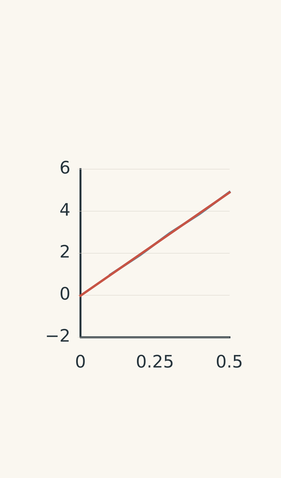
- Illustrative measured data
- Best-fit line; gradient = Δv/Δt
A straight-line fit to the illustrative data is approximately
\[ v=-0.02+9.82t \]
The small negative intercept comes from the scatter in the measurements. The gradient is approximately \(9.82\ \mathrm{m\\,s^{-2}}\), so the estimated gravitational acceleration is
\[ g\approx9.82\ \mathrm{m\\,s^{-2}} \]
The intercept is not the acceleration. It represents the velocity predicted by the fitted line at \(t=0\). In the ideal model, this should be zero because the object starts from rest.
Worked example: Estimate \(g\) from a velocity-time graph
A fitted velocity-time line passes through \((0.10\ \mathrm{s},\\,0.96\ \mathrm{m\\,s^{-1}})\) and \((0.50\ \mathrm{s},\\,4.89\ \mathrm{m\\,s^{-1}})\). Estimate \(g\) and check the units.
Step 1: Write the gradient formula.
\[ g=\frac{\Delta v}{\Delta t} \]
Step 2: Substitute the two points on the fitted line.
\[ \begin{aligned} g&=\frac{4.89-0.96}{0.50-0.10}\\[4pt] &=\frac{3.93\ \mathrm{m\\,s^{-1}}}{0.40\ \mathrm{s}}\\[4pt] &=9.825\ \mathrm{m\\,s^{-2}} \end{aligned} \]
Step 3: Interpret the result.
The estimated gravitational acceleration is approximately \(9.8\ \mathrm{m\\,s^{-2}}\). The units are correct because velocity is divided by time.
The two coordinates should be taken from the fitted line, not necessarily from the raw data points. Using points far apart reduces the effect of small errors when reading the gradient.
04Method 2: Find \(g\) from a displacement-versus-\(t^2\) graph
The second method uses the equation
\[ s=\frac12gt^2 \]
This equation is not linear when you plot displacement \(s\) against time \(t\). The displacement increases quadratically, producing a curve.
But look at what happens if you square every time measurement and plot \(s\) against \(t^2\) instead. The equation now has the form of a straight line.
Let \(m_s\) represent the gradient of the displacement-versus-\(t^2\) graph. Then
\[ m_s=\frac{g}{2} \]
Rearranging gives
\[ \boxed{g=2m_s} \]
The gradient is half the gravitational acceleration. Forgetting to multiply by two is a common source of an incorrect answer.
Why plotting against t² makes a straight line
| Left panel: displacement against time | s = ½gt² Horizontal axis: time t (s); vertical axis: displacement s (m). Upward-curving parabola: displacement increases quadratically with time. |
|---|---|
| Right panel: displacement against time squared | mₛ = g/2; g = 2mₛ Horizontal axis: time squared t² (s²); vertical axis: displacement s (m). Straight best-fit line; illustrative gradient ≈ 4.84 m/s², so g ≈ 9.68 m/s². |
How to construct the graph
- Calculate \(t^2\) for every time measurement.
- Put \(t^2\), in \(\mathrm{s^2}\), on the horizontal axis.
- Put displacement \(s\), in metres, on the vertical axis.
- Plot the data and draw a straight line of best fit.
- Calculate the gradient, then multiply it by two.
The gradient has units
\[ \frac{\mathrm{m}}{\mathrm{s^2}} =\mathrm{m\\,s^{-2}} \]
This is already the correct type of unit for acceleration. However, the gradient is \(g/2\), not \(g\), so you still need the final multiplication.
For the illustrative data, a straight-line fit is approximately
\[ s=0.005+4.84t^2 \]
The gradient is about \(4.84\ \mathrm{m\\,s^{-2}}\). Therefore,
\[ \begin{aligned} g&=2m_s\\ &=2(4.84\ \mathrm{m\\,s^{-2}})\\ &=9.68\ \mathrm{m\\,s^{-2}} \end{aligned} \]
This gives an estimate of \(9.68\ \mathrm{m\\,s^{-2}}\).
The small non-zero intercept is a reminder that experimental measurements rarely produce a perfect line through the origin. Ideally, displacement is zero when \(t=0\), provided you measure from the release point.
Worked example: Check a displacement-\(t^2\) result
A second experiment produces a best-fit gradient of \(4.86\ \mathrm{m\\,s^{-2}}\) on a graph of displacement against \(t^2\). Estimate \(g\) and calculate the percentage error relative to \(9.8\ \mathrm{m\\,s^{-2}}\).
Step 1: Convert the gradient into gravitational acceleration.
\[ \begin{aligned} g&=2m_s\\ &=2(4.86\ \mathrm{m\\,s^{-2}})\\ &=9.72\ \mathrm{m\\,s^{-2}} \end{aligned} \]
Step 2: Calculate the percentage error.
Use the accepted comparison value \(g=9.8\ \mathrm{m\\,s^{-2}}\).
\[ \begin{aligned} \%\text{ error} &=\frac{|g_{\text{measured}}-g_{\text{accepted}}|} {g_{\text{accepted}}}\times100\%\\[6pt] &=\frac{|9.72-9.8|}{9.8}\times100\%\\[6pt] &\approx0.82\% \end{aligned} \]
Step 3: Interpret the result.
The estimate is \(9.72\ \mathrm{m\\,s^{-2}}\), with a percentage error of approximately \(0.8\%\). It is close to the comparison value, but this alone does not establish how precise or reliable the experiment is.
05Which method should you use?
Both methods estimate the same physical quantity, but they respond differently to the way you collect data.
| Feature | Velocity-time graph | Displacement-\(t^2\) graph |
|---|---|---|
| Gradient represents | \(g\) | \(g/2\) |
| Final calculation | Use the gradient directly | Multiply the gradient by two |
| Initial velocity | Can be non-zero if acceleration is constant | Must be zero for this linear method |
| Main limitation | Calculated velocities can be noisy | Depends on accurate displacement and time measurements, and the release-from-rest condition |
| Useful when | Reliable velocity measurements are available | Position measurements are reliable and release from rest is controlled |
Neither method wins in every experiment.
Suppose you track a ball using video. Its positions may be relatively easy to measure, but calculating velocity from successive positions can amplify small errors. In that situation, the displacement-versus-\(t^2\) method may produce a steadier gradient.
Now suppose the ball is given a small downward push. The velocity-time graph can still provide \(g\), but the displacement-versus-\(t^2\) graph is no longer expected to be a straight line. The second method would be inappropriate unless you changed the model or analysis.
The sensible choice depends on the apparatus and the assumptions you can justify.
06How to check the accuracy of your result
Near Earth’s surface, gravitational acceleration is approximately \(9.8\ \mathrm{m\\,s^{-2}}\). Its exact value varies slightly with location, so use the value specified by your experiment or course when one is given.
For the illustrative data, the two methods gave:
| Method | Estimated \(g\) (\(\mathrm{m\\,s^{-2}}\)) | Percentage error relative to 9.8 |
|---|---|---|
| Velocity-time gradient | 9.82 | 0.2% |
| Displacement-\(t^2\) gradient | 9.68 | 1.2% |
The velocity-time result is closer to \(9.8\) for this particular data set. That does not prove the method is always more accurate. The data are illustrative, and the uncertainty of each fitted gradient has not yet been quantified.
Keep three ideas separate:
- Accuracy describes how close your result is to the accepted value.
- Precision describes the repeatability of measurements or results.
- Uncertainty describes the range of values reasonably consistent with the measurements and method.
A result can be precise but inaccurate if a systematic error affects every measurement. For example, a miscalibrated timer can produce consistent results that are all too high or too low.
Why the fitted gradient matters
Your gradient is an estimate, not an exact number. A slightly different line of best fit may produce a slightly different value of \(g\).
This is why drawing a sensible line matters. A line that is forced through every point will usually zigzag, while a line that ignores the trend will give a poor estimate.
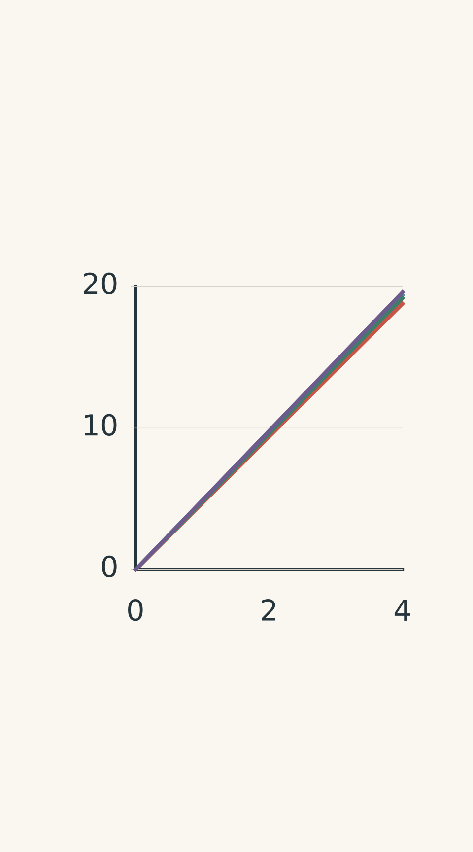
- Measured data (schematic)
- Shallowest: 4.7 m s⁻²; Δy = 14.1 m
- Best fit: 4.8 m s⁻²
- Steepest: 4.9 m s⁻²; Δy = 14.7 m
To assess the uncertainty in a gradient, you can draw the steepest and shallowest lines that are still reasonably consistent with the data, then calculate their gradients. The spread gives an estimate of the uncertainty in your slope.
For the displacement-versus-\(t^2\) method, remember that doubling the gradient also doubles its absolute uncertainty. For example, if \(m_s=4.8\pm0.1\ \mathrm{m\\,s^{-2}}\), then
\[ g=9.6\pm0.2\ \mathrm{m\\,s^{-2}} \]
A result reported as \(9.684273\ \mathrm{m\\,s^{-2}}\) would not be justified if the experiment only supports an uncertainty of several tenths of a metre per second squared.
Experimental limitations worth discussing
| Limitation | Why it matters | Practical improvement |
|---|---|---|
| Human reaction time | Starting and stopping a stopwatch introduces timing errors, especially during short falls. | Use a photogate or video with a known frame rate where possible. |
| Position uncertainty | Blur, parallax, and difficulty identifying the object’s centre affect displacement readings. | Align the camera perpendicular to the motion and place the ruler in the same plane as the object. |
| Velocity uncertainty | Calculating velocity from differences between noisy position measurements can amplify errors. | Use a suitable time interval, multiple measurements, and a fitted line. |
| Incorrect release conditions | An initial push invalidates the straight-line \(s\)-versus-\(t^2\) model. | Release the object gently from rest, or use the velocity-time method if the initial velocity is non-zero. |
| Poor gradient selection | Choosing two nearby raw data points can make the result very sensitive to measurement noise. | Use two well-separated points on the fitted line. |
Video setup for measuring gravitational acceleration
- Align the apparatus
Place the vertical metre ruler in the plane of the fall and mark the release point.
- Record the fall
Position the camera perpendicular to the plane; mark successive object positions at equal time intervals.
07A practical workflow for your next physics prac
You don’t need a perfect experiment to produce a useful result. You do need to understand which errors are likely to matter and how your analysis responds to them.
Before collecting data:
- Mark the release point so displacement is measured from a consistent origin.
- Use a known timing method, such as a photogate or calibrated video frame rate, if available.
- Release the object without deliberately pushing it.
- Repeat measurements where practical, rather than relying on a single fall.
When analysing your data:
- Keep the original measurements and avoid rounding intermediate values unnecessarily.
- Label both graph axes with the measured quantity and its units.
- Plot all the points and fit the appropriate line.
- Calculate the gradient using points far apart on that line.
- Apply the correct relationship: \(g=m_v\) for a velocity-time graph, or \(g=2m_s\) for a displacement-versus-\(t^2\) graph.
- Estimate uncertainty, compare your result with the accepted value, and identify the experimental limitation most likely to affect your result.
If you only have a hand stopwatch and the fall lasts a fraction of a second, reaction time may dominate the measurement. If you have reliable position tracking but noisy calculated velocities, the displacement method may be more useful. Your method should respond to the evidence you can actually collect.
08Questions and solutions
Question 1
A velocity-time graph uses upward as the positive direction. A dropped ball has a fitted gradient of \(-9.7\ \mathrm{m\\,s^{-2}}\). State the ball’s acceleration and the magnitude of gravitational acceleration. Explain the negative sign.
Solution 1
The ball’s acceleration is \(-9.7\ \mathrm{m\\,s^{-2}}\), and the magnitude of gravitational acceleration is \(9.7\ \mathrm{m\\,s^{-2}}\). The negative sign indicates that the acceleration points downwards, opposite to the chosen positive direction.
Acceleration is the gradient of a velocity-time graph. Because upward is positive, downward acceleration has a negative value. The gravitational acceleration has not become physically negative; only its signed component depends on the coordinate system.
Question 2
An object released from rest produces a displacement-versus-\(t^2\) graph with a best-fit gradient of \(4.72\ \mathrm{m\\,s^{-2}}\) and a vertical intercept of \(+0.030\ \mathrm{m}\).
Calculate \(g\). Explain whether the non-zero intercept proves that acceleration was not constant, and identify two possible causes of the intercept.
Solution 2
The estimated gravitational acceleration is \(9.44\ \mathrm{m\\,s^{-2}}\). The intercept does not, by itself, prove that the acceleration was non-constant.
For an object released from rest,
\[ s=\frac12gt^2 \]
Therefore, the gradient \(m_s\) is \(g/2\), giving
\[ \begin{aligned} g&=2m_s\\ &=2(4.72\ \mathrm{m\\,s^{-2}})\\ &=9.44\ \mathrm{m\\,s^{-2}} \end{aligned} \]
The units remain \(\mathrm{m\\,s^{-2}}\).
Ideally, the line passes through the origin because displacement is zero at \(t=0\). A non-zero intercept could arise because the displacement origin was set incorrectly, or because measurement scatter causes the fitted line not to pass through the origin.
The intercept is a reason to check the experimental setup, not proof that the physical model has failed. A substantial or systematic departure from the expected pattern deserves further investigation.
Question 3
Using the illustrative data table, the measured velocity points at \(t=0.20\ \mathrm{s}\) and \(t=0.30\ \mathrm{s}\) give a gradient of \(10.5\ \mathrm{m\\,s^{-2}}\). A best-fit line through all five points gives approximately \(9.82\ \mathrm{m\\,s^{-2}}\).
Which value is more defensible as the central estimate of \(g\)? Explain why the two results differ, and describe one method of estimating the uncertainty in your answer.
Solution 3
The best-fit gradient of approximately \(9.82\ \mathrm{m\\,s^{-2}}\) is the more defensible central estimate because it uses the overall trend of all five measurements rather than relying on just two adjacent points.
The adjacent-point calculation is
\[ \begin{aligned} g&=\frac{\Delta v}{\Delta t}\\ &=\frac{2.96-1.91}{0.30-0.20}\\ &=\frac{1.05\ \mathrm{m\\,s^{-1}}}{0.10\ \mathrm{s}}\\ &=10.5\ \mathrm{m\\,s^{-2}} \end{aligned} \]
The time interval is only \(0.10\ \mathrm{s}\). A small error in either velocity measurement can therefore produce a substantial change in the calculated gradient.
The best-fit line reduces the influence of individual fluctuations by using the overall pattern. To estimate uncertainty, draw the steepest and shallowest plausible lines consistent with the scatter and calculate both gradients. Their spread indicates how much the estimated acceleration could reasonably vary because of the fitting process.
Do not automatically average \(10.5\) and \(9.82\). The adjacent-point result is not an independent, equally reliable estimate simply because it is another number.
Question 4
A ball is launched gently downwards with an initial velocity of \(0.80\ \mathrm{m\\,s^{-1}}\). Its velocity-time graph is a straight line with a gradient of \(9.7\ \mathrm{m\\,s^{-2}}\).
A student also plots displacement \(s\) against \(t^2\) and doubles the gradient to calculate \(g\).
Is the student’s second method valid? Explain what each graph should look like and identify the more appropriate estimate of gravitational acceleration.
Solution 4
The student’s displacement-versus-\(t^2\) method is not valid for this motion, but the velocity-time gradient still gives \(g\approx9.7\ \mathrm{m\\,s^{-2}}\).
The initial velocity is \(u=0.80\ \mathrm{m\\,s^{-1}}\), so the velocity equation is
\[ v=0.80+9.7t \]
This is a straight line with gradient \(9.7\ \mathrm{m\\,s^{-2}}\). The non-zero initial velocity changes the intercept, not the gradient.
The displacement equation is different:
\[ s=0.80t+\frac12(9.7)t^2 \]
The \(0.80t\) term cannot be ignored. If we define \(x=t^2\), then \(t=\sqrt{x}\), giving
\[ s=0.80\sqrt{x}+4.85x \]
This is not a straight-line equation in \(x\), because it contains a square-root term. The displacement-versus-\(t^2\) graph will not have a constant gradient.
The tempting approach is to apply \(g=2m_s\) to any falling object. The missing condition is that the object must start from rest. Here, the velocity-time gradient is the appropriate method, assuming acceleration remains constant and the measurements are reliable.
Question 5
An object is tracked on video. Assume it is released from rest, air resistance is negligible, and the position measurements are accurate.
The group suspects a timing-scale error. To test the effect, suppose the displayed elapsed time \(T\) is \(3\%\) larger than the true elapsed time \(t\):
\[ T=1.03t \]
The software also calculates velocity from those same displayed time intervals, so its measured velocity is \(v_m=\Delta s/\Delta T\).
The group reports \(g_v=9.2\ \mathrm{m\\,s^{-2}}\) from the velocity-versus-\(T\) graph and \(g_s=9.8\ \mathrm{m\\,s^{-2}}\) from the displacement-versus-\(T^2\) graph.
Using \(9.8\ \mathrm{m\\,s^{-2}}\) as the true value, determine what a \(3\%\) timing-scale error alone would predict for each graph. Can this error alone explain the two reported results? Justify your conclusion.
Solution 5
No. A constant timing-scale error of this type should cause both methods to estimate the same value of \(g\), approximately \(9.24\ \mathrm{m\\,s^{-2}}\). It cannot, by itself, explain why one graph gives \(9.2\) while the other gives \(9.8\ \mathrm{m\\,s^{-2}}\).
The crucial detail is that the timing error affects both the horizontal axis and the calculated velocity values.
Let \(k=1.03\), so that \(T=kt\).
Step 1: Work out the effect on the velocity-time graph.
The true velocity is
\[ v=gt \]
Because the software calculates velocity using the displayed time intervals, the measured velocity is
\[ v_m=\frac{v}{k} \]
Since \(t=T/k\),
\[ v_m=\frac{gT}{k^2} \]
The gradient of the measured velocity-versus-\(T\) graph is therefore
\[ g_v=\frac{g}{k^2} \]
Step 2: Work out the effect on the displacement-versus-\(T^2\) graph.
The true displacement is
\[ s=\frac12gt^2 \]
Substituting \(t=T/k\) gives
\[ s=\frac{g}{2k^2}T^2 \]
The gradient of the displacement-versus-\(T^2\) graph is \(g/(2k^2)\). Doubling it produces
\[ g_s=\frac{g}{k^2} \]
Both methods therefore have the same timing-scale dependence.
Step 3: Calculate the predicted results.
Using \(g=9.8\ \mathrm{m\\,s^{-2}}\),
\[ \begin{aligned} g_v=g_s &=\frac{9.8}{(1.03)^2}\\[4pt] &=\frac{9.8}{1.0609}\\[4pt] &\approx9.24\ \mathrm{m\\,s^{-2}} \end{aligned} \]
The predicted value is approximately \(9.24\ \mathrm{m\\,s^{-2}}\) for both methods. The velocity-time estimate of \(9.2\) is consistent with that prediction to the precision reported, but the displacement-based estimate of \(9.8\) is not.
Step 4: Interpret the disagreement.
A \(3\%\) timing-scale error could explain why both estimates are lower than the true value, but it cannot explain the disagreement between the two methods. If the assumptions hold, at least one additional issue must be affecting the results, such as measurement scatter, inconsistent data processing, or an error in fitting a gradient.
There is another important limitation: both graphs use the same underlying position and time data, so agreement between them is not necessarily independent confirmation.
The next defensible step is to check the timing calibration, inspect the fitted lines, and estimate the uncertainty in both gradients. Only then can you decide whether the difference between the two estimates is meaningful or simply a consequence of measurement uncertainty.