
Measuring Stellar Motion with Doppler Shifts: HSC Physics
Learn how spectral line shifts reveal stellar radial velocity, while line broadening can reveal projected rotational velocity. Includes worked examples and challenging HSC-style questions.
A hydrogen absorption line that sits at \(656.3\) nm in the laboratory appears at a slightly different wavelength in a star. That shift can tell us how fast the star is moving towards or away from us. But suppose the same line is also noticeably wider than the laboratory line. Is that just a messier measurement, or is the star telling us something else?
Predict first: if the whole star moves directly away from Earth, should its spectral line mainly move sideways on a wavelength graph, or become wider?
It mainly moves sideways. If the star rotates, though, different parts of its surface move towards and away from us at the same time. Their slightly different Doppler shifts pile together, producing a broadened line.
That gives us two separate clues from one spectrum: line shift can reveal radial velocity, while line broadening can reveal projected rotational velocity.
01Two motions leave different fingerprints
Imagine an unresolved star as a tiny spinning disc.
If the whole star is moving away from Earth, every visible part shares that overall motion. Its spectral lines are shifted towards longer wavelengths. If the star moves towards us, they shift towards shorter wavelengths.
Rotation is different. One side of the spinning star moves partly towards us, while the opposite side moves partly away.
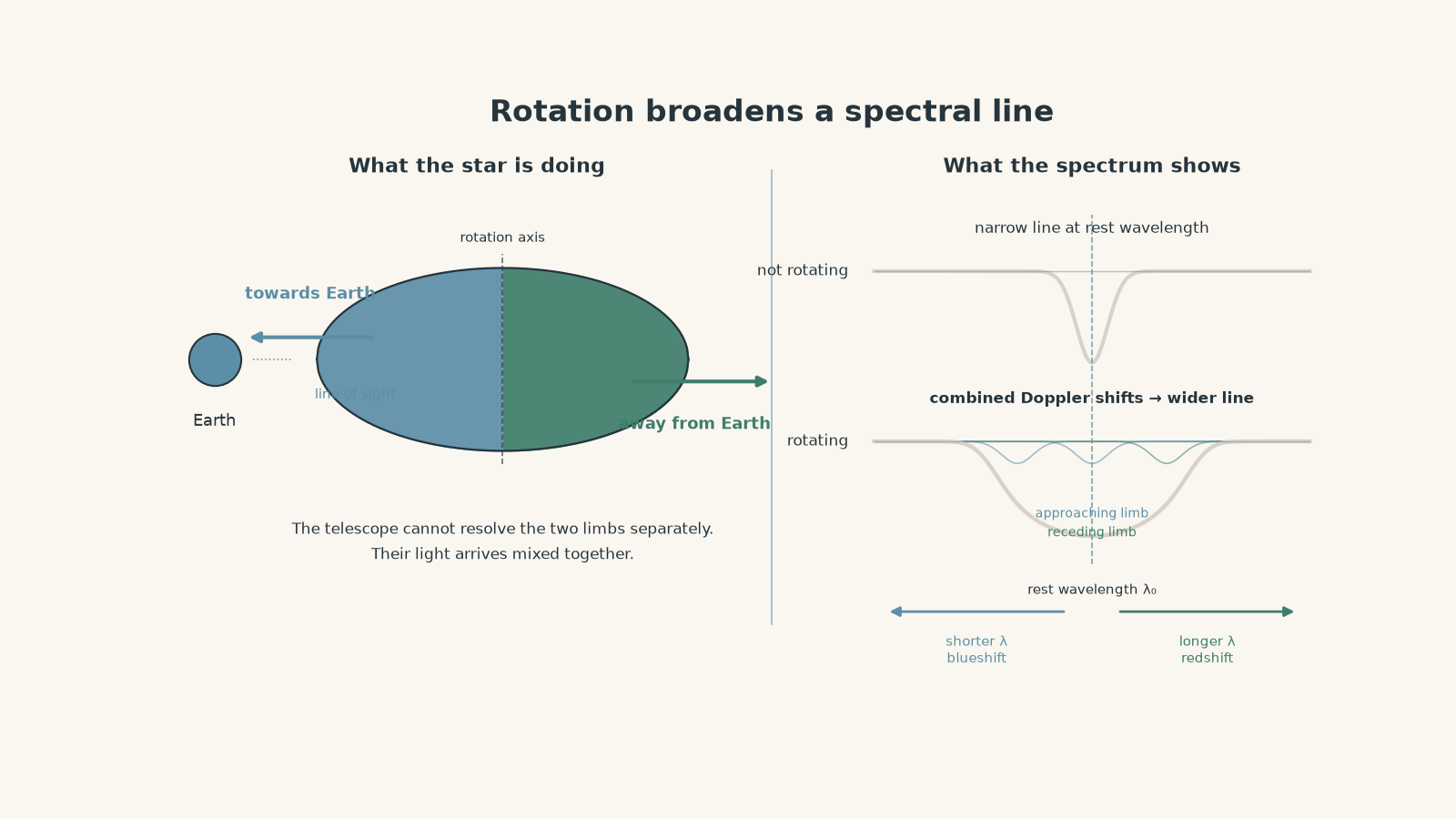
The approaching side produces a small blueshift. The receding side produces a small redshift. Regions between those two extremes have intermediate line-of-sight velocities, so they produce intermediate shifts.
A telescope generally cannot separate all those patches on a distant star. It collects their light together. The result is not a neat collection of separate lines. It is one broadened spectral line.
A useful first model is therefore:
| What happens to the spectral line? | First interpretation |
|---|---|
| Whole line moves to longer wavelength | Star has radial motion away from us |
| Whole line moves to shorter wavelength | Star has radial motion towards us |
| Line becomes wider | Different visible regions have different radial velocities |
| Line is shifted and broadened | The star can have both radial motion and rotation |
The word “first” matters. Broadening is not caused only by rotation. Temperature, gas motion, pressure effects, and the measuring instrument can also widen spectral lines. We can infer rotation only when rotational broadening has been identified or the other contributions have been accounted for.
If you need a refresher on where absorption and emission lines come from, read Continuous, Emission and Absorption Spectra: HSC Physics.
02Radial velocity comes from the position of the line
Suppose a particular element produces a line at laboratory wavelength \(\lambda_0\). We observe the same line from a star at wavelength \(\lambda_{\text{obs}}\).
The wavelength change is
\[
\Delta \lambda = \lambda_{\text{obs}}-\lambda_0
\]
where:
- \(\lambda_0\) is the wavelength measured for the stationary laboratory source,
- \(\lambda_{\text{obs}}\) is the wavelength observed from the star, and
- \(\Delta\lambda\) is the Doppler shift.
For speeds much smaller than the speed of light, the HSC-useful Doppler relationship is
\[
\frac{v_r}{c}\approx\frac{\Delta\lambda}{\lambda_0}
\]
so
\[
v_r\approx c\frac{\Delta\lambda}{\lambda_0}
\]
Here \(v_r\) is the star’s radial velocity and \(c=3.00\times10^8\) m/s is the speed of light.
We’ll use the sign convention:
- \(v_r>0\): moving away from us, so the line is redshifted;
- \(v_r<0\): moving towards us, so the line is blueshifted.
Why “radial” velocity rather than simply “velocity”?
Because spectroscopy only measures the component of motion along our line of sight. A star could also be moving sideways across the sky. That sideways component does not produce this simple Doppler shift.
Worked example: Finding a star’s radial velocity
A hydrogen line has a laboratory wavelength of \(656.28\) nm. In a star’s spectrum, the centre of the line occurs at \(656.34\) nm. Determine the star’s radial velocity.
Step 1
\[
\Delta\lambda=656.34-656.28=0.06\text{ nm}
\]
The shift is positive, so we already expect the star to be moving away.
Step 2
Because the numerator and denominator are both in nanometres, their units cancel.
\[
\begin{aligned}
v_r
&=c\frac{\Delta\lambda}{\lambda_0}\\
&=(3.00\times10^8)\frac{0.06}{656.28}\\
&=2.74\times10^4\text{ m/s}
\end{aligned}
\]
Step 3
\[
v_r=27.4\text{ km/s away from Earth}
\]
This does not mean the star’s total speed through space is \(27.4\) km/s. It means the component of its velocity along our line of sight is \(27.4\) km/s away from us.
03Rotation changes the width, not just the centre
Now picture the same star spinning.
Let its equatorial rotational speed be \(v_{\text{eq}}\). Unless we are looking exactly down its rotation axis, one edge has a component of rotational velocity towards us and the opposite edge has one away from us.
So why doesn’t the blueshift from one side simply cancel the redshift from the other?
Because the telescope adds light intensities, not wavelength shifts. One part of the star contributes absorption at a slightly shorter wavelength, another contributes absorption at a slightly longer wavelength, and other regions contribute wavelengths between them. Those contributions overlap into a wider absorption feature.
It’s a little like ten people trying to sing the same note while some are on a moving walkway coming towards you and others are travelling away. The original note has not changed, but you receive a spread of Doppler-shifted versions. The analogy stops being exact because a stellar line profile depends on the brightness and velocity of different parts of the stellar surface, as well as other broadening mechanisms.
The inclination problem
There is one important complication.
Suppose a star rotates rapidly, but its rotation axis points almost directly at Earth. Most of the surface motion is then sideways from our point of view. The line-of-sight components are small, so the rotational broadening can also be small.
Define \(i\) as the angle between the rotation axis and our line of sight.
- \(i=0^\circ\): we see the star nearly pole-on.
- \(i=90^\circ\): we see it equator-on.
Spectral broadening therefore normally gives
\[
v_{\text{eq}}\sin i
\]
rather than \(v_{\text{eq}}\) by itself.
This quantity is called the projected rotational velocity.
So a narrow line does not prove that a star rotates slowly. It could be rotating quickly while viewed nearly pole-on.
04Separating shift from broadening
For an idealised broadened line, suppose its rotationally broadened blue and red limits are \(\lambda_{\text{blue}}\) and \(\lambda_{\text{red}}\).
The centre is approximately
\[
\lambda_c=\frac{\lambda_{\text{red}}+\lambda_{\text{blue}}}{2}
\]
The movement of this centre away from the laboratory wavelength tells us the radial velocity:
\[
v_r\approx c\frac{\lambda_c-\lambda_0}{\lambda_0}
\]
The rotational half-width is
\[
\Delta\lambda_{\text{rot}}
=\frac{\lambda_{\text{red}}-\lambda_{\text{blue}}}{2}
\]
and, in the same low-speed approximation,
\[
v_{\text{eq}}\sin i
\approx
c\frac{\Delta\lambda_{\text{rot}}}{\lambda_0}
\]
or
\[
v_{\text{eq}}\sin i
\approx
c\frac{\lambda_{\text{red}}-\lambda_{\text{blue}}}{2\lambda_0}
\]
These equations are an idealised way of representing rotational broadening. Real spectral lines do not usually have perfectly sharp “edges”, so astronomers analyse the shape of the whole line profile and account for other broadening mechanisms.
For HSC reasoning, the essential distinction is simpler:
- use the centre of the line to investigate bulk radial motion;
- use the spread around the centre to investigate rotation.
Worked example: A rotating and receding star
A spectral line has a laboratory wavelength of \(500.00\) nm. After other important broadening effects have been accounted for, its rotational profile extends approximately from \(500.08\) nm to \(500.32\) nm.
Determine the star’s radial velocity and projected rotational velocity.
Step 1
\[
\lambda_c=\frac{500.08+500.32}{2}=500.20\text{ nm}
\]
The centre is redshifted by
\[
\Delta\lambda=500.20-500.00=0.20\text{ nm}
\]
Step 2
\[
\begin{aligned}
v_r
&=c\frac{0.20}{500.00}\\
&=(3.00\times10^8)\frac{0.20}{500.00}\\
&=1.20\times10^5\text{ m/s}
\end{aligned}
\]
So the star is moving away from us at
\[
v_r=120\text{ km/s}
\]
Step 3
\[
\Delta\lambda_{\text{rot}}
=\frac{500.32-500.08}{2}
=0.12\text{ nm}
\]
Step 4
\[
\begin{aligned}
v_{\text{eq}}\sin i
&=c\frac{0.12}{500.00}\\
&=(3.00\times10^8)\frac{0.12}{500.00}\\
&=7.20\times10^4\text{ m/s}
\end{aligned}
\]
Therefore,
\[
v_{\text{eq}}\sin i=72.0\text{ km/s}
\]
The spectrum tells us that the star is receding at \(120\) km/s and has a projected rotational velocity of \(72.0\) km/s.
If another observation told us that \(i=30^\circ\), then
\[
72.0=v_{\text{eq}}\sin30^\circ
\]
so
\[
v_{\text{eq}}=144\text{ km/s}
\]
Without that inclination information, \(72.0\) km/s is not the true equatorial rotational speed. It is the projected value.
05The most tempting mistakes
Mistake 1: “A redshifted line means the whole star looks red”
Not necessarily.
The wavelength changes involved can be tiny compared with the width of the visible spectrum. We usually identify Doppler motion by measuring known spectral lines precisely, not by deciding that the star looks visibly redder or bluer.
That requires knowing which line you are looking at in the first place. Identifying Elements with Spectral Lines: HSC Physics explains how the line pattern acts as an elemental fingerprint.
Mistake 2: “A wider line automatically means faster rotation”
No.
Rotation can broaden spectral lines, but so can thermal motion and other physical or instrumental effects. A claim about rotational velocity needs the rotational contribution to the broadening to be isolated or justified.
Mistake 3: “The reddest part of the line gives the star’s radial velocity”
This is especially tempting.
For a rotating star, the reddest edge includes both the whole star’s radial motion and the extra recession of the rotating limb. The bluest edge includes the radial motion and the approaching limb’s rotational contribution.
The centre isolates the bulk motion. The half-width isolates the opposing rotational motions.
Mistake 4: “Every Doppler-shifted line moves by the same number of nanometres”
The important quantity is the fractional shift,
\[
\frac{\Delta\lambda}{\lambda_0}
\]
not \(\Delta\lambda\) alone.
If one line at \(400\) nm and another at \(600\) nm come from the same moving star, the \(600\) nm line should have a larger wavelength shift in nanometres for the same radial velocity.
Mistake 5: “Spectroscopy gives the full rotation speed”
Usually it gives \(v_{\text{eq}}\sin i\).
That hidden \(\sin i\) is one of the most important limitations of the measurement.
06A compact decision method
When you are given a stellar spectrum problem, work in this order.
- Identify the laboratory wavelength \(\lambda_0\).
- Find the centre of the observed line.
- Compare the centre with \(\lambda_0\) to determine radial velocity.
- Find the line’s half-width if rotational broadening information is provided.
- Convert that half-width into \(v_{\text{eq}}\sin i\).
- Only calculate \(v_{\text{eq}}\) itself if the inclination \(i\), or equivalent information, is known.
- Check that the question has justified treating the width as rotational broadening.
The order matters. If you start by treating the red edge as the radial Doppler shift, rotation contaminates your result.
07Questions and solutions
Question 1
A spectral line has a laboratory wavelength of \(486.1\) nm. In a star’s spectrum, the centre of the line is measured at \(486.3\) nm.
Calculate the star’s radial velocity and state whether it is moving towards or away from Earth.
Solution 1
The star is moving away from Earth at approximately \(123\) km/s.
The observed wavelength is larger than the laboratory wavelength, so the line is redshifted.
First find the shift:
\[
\Delta\lambda=486.3-486.1=0.2\text{ nm}
\]
Then use
\[
v_r=c\frac{\Delta\lambda}{\lambda_0}
\]
Substituting,
\[
\begin{aligned}
v_r
&=(3.00\times10^8)\frac{0.2}{486.1}\\
&=1.23\times10^5\text{ m/s}\\
&=123\text{ km/s}
\end{aligned}
\]
The positive shift means recession.
A tempting mistake is to describe \(123\) km/s as the star’s total velocity. It is only its radial component relative to the observer.
Question 2
A line with laboratory wavelength \(656.3\) nm is broadened by stellar rotation. Its rotational profile extends from \(656.12\) nm to \(656.56\) nm.
Assume other broadening effects have already been accounted for.
Calculate:
a. the radial velocity of the star,
b. the projected rotational velocity \(v_{\text{eq}}\sin i\), and
c. explain why using \(656.56\) nm directly as the star’s Doppler-shifted wavelength would give the wrong radial velocity.
Solution 2
The star is receding at approximately \(18.3\) km/s, while its projected rotational velocity is approximately \(101\) km/s. The red edge cannot be used directly for radial velocity because it contains both the bulk recession and the rotational motion of the receding limb.
For part a, first find the line centre:
\[
\lambda_c=\frac{656.12+656.56}{2}=656.34\text{ nm}
\]
The centre has shifted by
\[
\Delta\lambda=656.34-656.30=0.04\text{ nm}
\]
Therefore,
\[
\begin{aligned}
v_r
&=(3.00\times10^8)\frac{0.04}{656.3}\\
&=1.83\times10^4\text{ m/s}\\
&=18.3\text{ km/s}
\end{aligned}
\]
For part b, the rotational half-width is
\[
\Delta\lambda_{\text{rot}}
=\frac{656.56-656.12}{2}
=0.22\text{ nm}
\]
So
\[
\begin{aligned}
v_{\text{eq}}\sin i
&=(3.00\times10^8)\frac{0.22}{656.3}\\
&=1.01\times10^5\text{ m/s}\\
&=101\text{ km/s}
\end{aligned}
\]
For part c, \(656.56\) nm comes from the extreme red side of the rotationally broadened profile. That part of the star is receding because of rotation as well as sharing the star’s overall radial velocity.
The tempting route is to calculate
\[
c\frac{656.56-656.30}{656.30}
\]
and call that the radial velocity. Doing so mixes two different motions. The midpoint of the line, not its reddest edge, represents the bulk radial shift.
Question 3
Two identified spectral lines from the same star have these laboratory and observed centre wavelengths:
| Line | Laboratory wavelength | Observed centre |
|---|---|---|
| A | \(400.00\) nm | \(399.92\) nm |
| B | \(600.00\) nm | \(599.88\) nm |
After other sources of broadening are removed, line A has a rotational full width of \(0.24\) nm and line B has a rotational full width of \(0.36\) nm.
Determine whether the two lines are consistent with one radial velocity and one projected rotational velocity. Calculate both velocities.
Solution 3
Yes. Both lines are consistent with a radial velocity of \(60.0\) km/s towards Earth and a projected rotational velocity of \(90.0\) km/s.
For line A, the centre shift is
\[
\Delta\lambda_A=399.92-400.00=-0.08\text{ nm}
\]
so
\[
\begin{aligned}
v_{r,A}
&=(3.00\times10^8)\frac{-0.08}{400.00}\\
&=-6.00\times10^4\text{ m/s}\\
&=-60.0\text{ km/s}
\end{aligned}
\]
For line B,
\[
\Delta\lambda_B=599.88-600.00=-0.12\text{ nm}
\]
and
\[
\begin{aligned}
v_{r,B}
&=(3.00\times10^8)\frac{-0.12}{600.00}\\
&=-6.00\times10^4\text{ m/s}\\
&=-60.0\text{ km/s}
\end{aligned}
\]
The shifts are different in nanometres, but their fractional shifts are the same.
Now consider rotation.
Line A has half-width
\[
\Delta\lambda_{\text{rot},A}=\frac{0.24}{2}=0.12\text{ nm}
\]
so
\[
\begin{aligned}
v_{\text{eq}}\sin i
&=(3.00\times10^8)\frac{0.12}{400.00}\\
&=9.00\times10^4\text{ m/s}\\
&=90.0\text{ km/s}
\end{aligned}
\]
Line B has half-width
\[
\Delta\lambda_{\text{rot},B}=\frac{0.36}{2}=0.18\text{ nm}
\]
giving
\[
\begin{aligned}
v_{\text{eq}}\sin i
&=(3.00\times10^8)\frac{0.18}{600.00}\\
&=9.00\times10^4\text{ m/s}\\
&=90.0\text{ km/s}
\end{aligned}
\]
Again, the widths in nanometres are different, but the fractional widths are equal.
The tempting conclusion is that the two lines disagree because \(0.08\neq0.12\) and \(0.24\neq0.36\). That compares absolute wavelength changes. Doppler motion is connected to fractional wavelength change, so both measurements describe the same motions.
Question 4
A star has radius \(6.0\times10^8\) m and completes one rotation every \(10.0\) hours.
An absorption line with laboratory wavelength \(550.00\) nm has rotational limits at \(550.055\) nm and \(550.165\) nm. Assume all non-rotational broadening has been removed.
Determine:
a. the star’s radial velocity,
b. its projected rotational velocity,
c. its equatorial rotational speed using its radius and period, and
d. the approximate inclination \(i\) of its rotation axis to our line of sight.
Explain why describing the star as a “slow rotator” from the spectral width alone would be misleading.
Solution 4
The star is receding at \(60.0\) km/s, has a projected rotational velocity of \(30.0\) km/s, but actually rotates at about \(105\) km/s at its equator. Its rotation axis is inclined by only about \(17^\circ\) to our line of sight.
For part a, the line centre is
\[
\lambda_c=\frac{550.055+550.165}{2}=550.110\text{ nm}
\]
so
\[
\Delta\lambda=550.110-550.000=0.110\text{ nm}
\]
Therefore,
\[
\begin{aligned}
v_r
&=(3.00\times10^8)\frac{0.110}{550.00}\\
&=6.00\times10^4\text{ m/s}\\
&=60.0\text{ km/s}
\end{aligned}
\]
For part b, the rotational half-width is
\[
\Delta\lambda_{\text{rot}}
=\frac{550.165-550.055}{2}
=0.055\text{ nm}
\]
Thus,
\[
\begin{aligned}
v_{\text{eq}}\sin i
&=(3.00\times10^8)\frac{0.055}{550.00}\\
&=3.00\times10^4\text{ m/s}\\
&=30.0\text{ km/s}
\end{aligned}
\]
For part c, the equatorial point travels one circumference every rotation:
\[
v_{\text{eq}}=\frac{2\pi R}{T}
\]
The period is
\[
T=10.0\times3600=3.60\times10^4\text{ s}
\]
so
\[
\begin{aligned}
v_{\text{eq}}
&=\frac{2\pi(6.0\times10^8)}{3.60\times10^4}\\
&=1.05\times10^5\text{ m/s}\\
&=105\text{ km/s}
\end{aligned}
\]
For part d,
\[
v_{\text{eq}}\sin i=30.0\text{ km/s}
\]
so
\[
\sin i=\frac{30.0}{105}=0.286
\]
and therefore
\[
i\approx17^\circ
\]
The tempting interpretation is that the modest line width proves a modest true rotation speed. The independent radius and period show otherwise. The star is rotating at about \(105\) km/s, but we are viewing it fairly close to its pole, so only about \(30\) km/s of the equatorial velocity appears along our line of sight.
This is exactly why spectroscopy by itself normally gives \(v_{\text{eq}}\sin i\), not \(v_{\text{eq}}\).
Question 5
A rotating star produces two spectral lines. Other sources of broadening have been removed.
For a line with laboratory wavelength \(500.00\) nm, the rotational profile extends from \(500.00\) nm to \(500.40\) nm.
For another line with laboratory wavelength \(650.00\) nm, the profile extends from \(650.00\) nm to \(650.52\) nm.
A student argues:
Neither line extends to a wavelength shorter than its laboratory wavelength, so no visible part of the star is moving towards us. The broadening therefore cannot be due to rotation.
The star has radius \(7.0\times10^8\) m and rotation period \(5.1\) hours.
Determine the radial velocity, projected rotational velocity, and approximate inclination of the star. Then explain precisely what is wrong with the student’s argument.
Solution 5
The star is receding at approximately \(120\) km/s, its projected rotational velocity is also approximately \(120\) km/s, and its rotation axis is inclined by about \(30^\circ\) to our line of sight. The approaching limb really is moving towards us relative to the star’s centre, but its rotational blueshift almost exactly cancels the star’s overall redshift.
Start with the \(500.00\) nm line.
Its observed centre is
\[
\lambda_c=\frac{500.00+500.40}{2}=500.20\text{ nm}
\]
so the centre has shifted by
\[
\Delta\lambda=0.20\text{ nm}
\]
The radial velocity is therefore
\[
\begin{aligned}
v_r
&=(3.00\times10^8)\frac{0.20}{500.00}\\
&=1.20\times10^5\text{ m/s}\\
&=120\text{ km/s}
\end{aligned}
\]
The rotational half-width is also
\[
\Delta\lambda_{\text{rot}}
=\frac{500.40-500.00}{2}
=0.20\text{ nm}
\]
so
\[
\begin{aligned}
v_{\text{eq}}\sin i
&=(3.00\times10^8)\frac{0.20}{500.00}\\
&=120\text{ km/s}
\end{aligned}
\]
The \(650.00\) nm line confirms the result.
Its centre is
\[
\lambda_c=\frac{650.00+650.52}{2}=650.26\text{ nm}
\]
giving
\[
\frac{0.26}{650.00}=4.00\times10^{-4}
\]
and therefore
\[
v_r=120\text{ km/s}
\]
Its half-width is
\[
\frac{0.52}{2}=0.26\text{ nm}
\]
which gives the same projected rotational velocity:
\[
v_{\text{eq}}\sin i=120\text{ km/s}
\]
Now use the independent radius and period to find the true equatorial speed.
Convert the period:
\[
T=5.1\times3600=1.836\times10^4\text{ s}
\]
Then
\[
\begin{aligned}
v_{\text{eq}}
&=\frac{2\pi R}{T}\\
&=\frac{2\pi(7.0\times10^8)}{1.836\times10^4}\\
&\approx2.40\times10^5\text{ m/s}\\
&\approx240\text{ km/s}
\end{aligned}
\]
Since
\[
v_{\text{eq}}\sin i=120\text{ km/s}
\]
we have
\[
\sin i=\frac{120}{240}=0.500
\]
so
\[
i\approx30^\circ
\]
Now for the apparent contradiction.
At the approaching limb, the star’s overall radial motion and its rotational motion act in opposite directions. To first order, its line-of-sight velocity is approximately
\[
v_{\text{limb}}\approx v_r-v_{\text{eq}}\sin i
\]
Here,
\[
v_{\text{limb}}\approx120-120=0\text{ km/s}
\]
So the rotationally approaching limb does produce a blueshift relative to the centre of the star’s spectrum. But the entire star is already redshifted because it is receding at \(120\) km/s. The two effects cancel at that edge, placing it back at approximately the laboratory wavelength.
On the opposite limb, they add:
\[
v_{\text{limb}}\approx120+120=240\text{ km/s away}
\]
which produces the strongly redshifted edge.
The student’s mistake is treating “not blueshifted relative to the laboratory” as equivalent to “not moving towards us because of rotation”. Those are different comparisons. Rotation must be considered relative to the star’s bulk radial motion.
That is the deeper use of spectral lines: a single profile can contain several motions at once. Once you learn to separate its centre from its width, you can extract the motion of the star as a whole from the motion of its surface. The next step is to separate motion from the other information hiding in the same spectrum, including temperature, which is explored in Finding Stellar Temperature from Spectra: HSC Physics.