
Why Half-Life Does Not Predict When One Nucleus Will Decay
Half-life does not tell you when an individual nucleus will decay. Learn how radioactive decay behaves statistically, use a coin-toss model to understand sample fluctuations, interpret half-life graphs, and solve HSC Physics questions with worked examples.
You write, “The half-life is 6 hours, so every nucleus decays after 6 hours.” Then you predict that after three half-lives, the sample must be empty. This is a common radioactive-decay mistake: you’ve turned a statistical pattern for a population into a countdown for each individual nucleus.
Before going further, predict what remains from a sample of 800 undecayed nuclei after one half-life. The expected number is 400, but a real measurement might find 392 or 407. Half-life predicts the statistical behaviour of the sample, not the exact moment each nucleus decays.
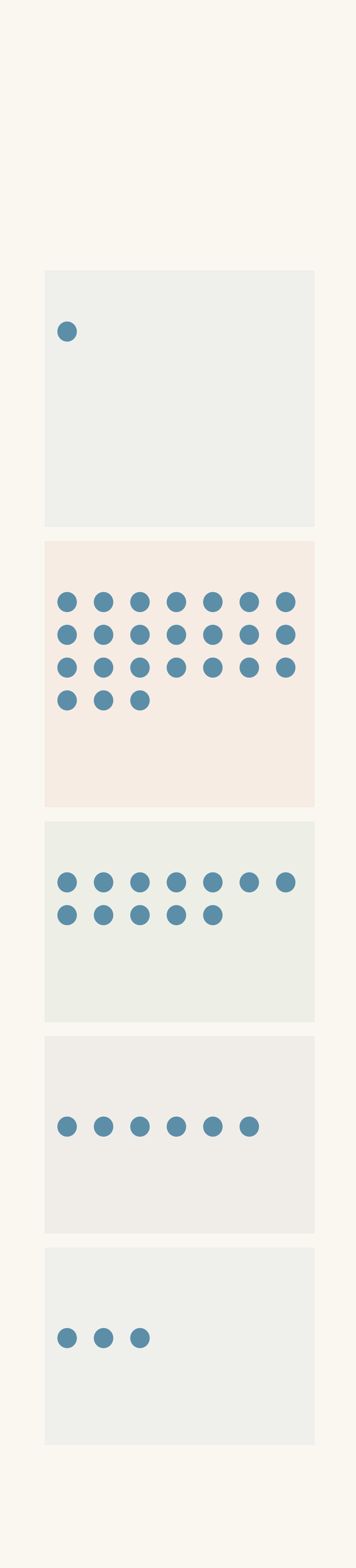
- Undecayed nucleus
01The mistake: treating half-life as a timer
A half-life, written \(T_{1/2}\), is the time over which the expected number of undecayed nuclei in a radioactive sample falls to half its previous value.
The key word is expected.
For a particular nucleus, we cannot predict its exact decay time from the half-life alone. If the nucleus is still undecayed at the start of an interval lasting one half-life, it has a 50% probability of decaying during that interval.
Suppose an isotope has a half-life of 6 hours.
- A nucleus that has survived for 1 hour has a 50% probability of decaying during the next 6 hours.
- A nucleus that has survived for 20 hours also has a 50% probability of decaying during the next 6 hours.
- Neither nucleus is guaranteed to decay during that interval.
The second nucleus is not overdue. Surviving for a long time does not make its next decay inevitable.
This is the distinction to remember: half-life describes a probability for individual nuclei and a predictable statistical pattern for the sample.
02Model radioactive decay with a coin toss
Radioactive decay is difficult to picture because we cannot see a nucleus waiting to decay. A coin-toss model gives us a practical way to explore the statistics.
Imagine that each coin represents one radioactive nucleus.
- Heads: the nucleus decays during the next half-life interval, so remove the coin.
- Tails: the nucleus survives, so keep the coin.
- Repeat the process with the surviving coins.
Each fair coin has a 50% probability of being removed in each round. This represents the 50% probability that a surviving nucleus decays during the next half-life interval.
Start with 64 coins. What do you expect after three rounds?
| Elapsed time | Expected survivors | One possible run |
|---|---|---|
| 0 half-lives | 64 | 64 |
| 1 half-life | 32 | 35 |
| 2 half-lives | 16 | 18 |
| 3 half-lives | 8 | 9 |
The expected counts are averages across many equivalent trials. The final column shows one possible outcome, not a prediction that every run must follow.
In this example, the actual number surviving after the first round is 35 rather than 32. After the second round, 18 survive rather than the original sample’s expected count of 16. The result still follows the model: each surviving coin gets another independent chance of being removed.
Expected decay versus one possible run
| Expected count | 0, 1, 2, 3 half-lives: 64, 32, 16, 8 nuclei. |
|---|---|
| One possible run | 0, 1, 2, 3 half-lives: 64, 35, 18, 9 nuclei. |
Why repeated trials fluctuate
Suppose you repeat the coin-toss experiment ten times, always starting with 16 coins.
You will not necessarily get eight survivors in every trial. You might get five in one trial, eight in another, and eleven in a third.
That variation is not a failure of the model. The model predicts a 50% survival probability, not exactly 50% survival in every small group.
If you repeat the experiment many times, the average number of survivors approaches the expected value. If you start with a much larger number of coins, the fraction surviving will generally stay closer to 50% in each round.
There is an important distinction here. A large sample can have larger fluctuations in its absolute number of survivors while having smaller fluctuations in its fraction surviving.
The coin analogy has one limitation: coins make their decision only when tossed, whereas radioactive nuclei can decay at any time. The model represents survival probabilities at half-life intervals. It does not describe the physical mechanism or exact timing of an individual decay.
03What a half-life graph actually shows
The coin model gives us a pattern. A half-life graph expresses that pattern mathematically.
For a sample with an initial number of undecayed nuclei \(N_0\), the expected number remaining after time \(t\) is
\[ N_{\text{expected}}(t) = N_0\left(\frac12\right)^{t/T_{1/2}} \]
Here:
- \(N_{\text{expected}}\) is the expected number of undecayed nuclei at time \(t\).
- \(N_0\) is the initial number of undecayed nuclei.
- \(t\) is the elapsed time.
- \(T_{1/2}\) is the half-life.
The exponent \(t/T_{1/2}\) tells you how many half-lives have elapsed. It does not count how many times each nucleus has been given a countdown.
Consider a sample that starts with 800 undecayed nuclei.
| Elapsed time | Expected fraction remaining | Expected number remaining |
|---|---|---|
| \(0\) | \(1\) | 800 |
| \(T_{1/2}\) | \(1/2\) | 400 |
| \(2T_{1/2}\) | \(1/4\) | 200 |
| \(3T_{1/2}\) | \(1/8\) | 100 |
| \(4T_{1/2}\) | \(1/16\) | 50 |
Notice what happens after three half-lives. The expected number remaining is 100, not zero.
Each half-life halves the expected number that remains. It does not remove half of the original sample every time.
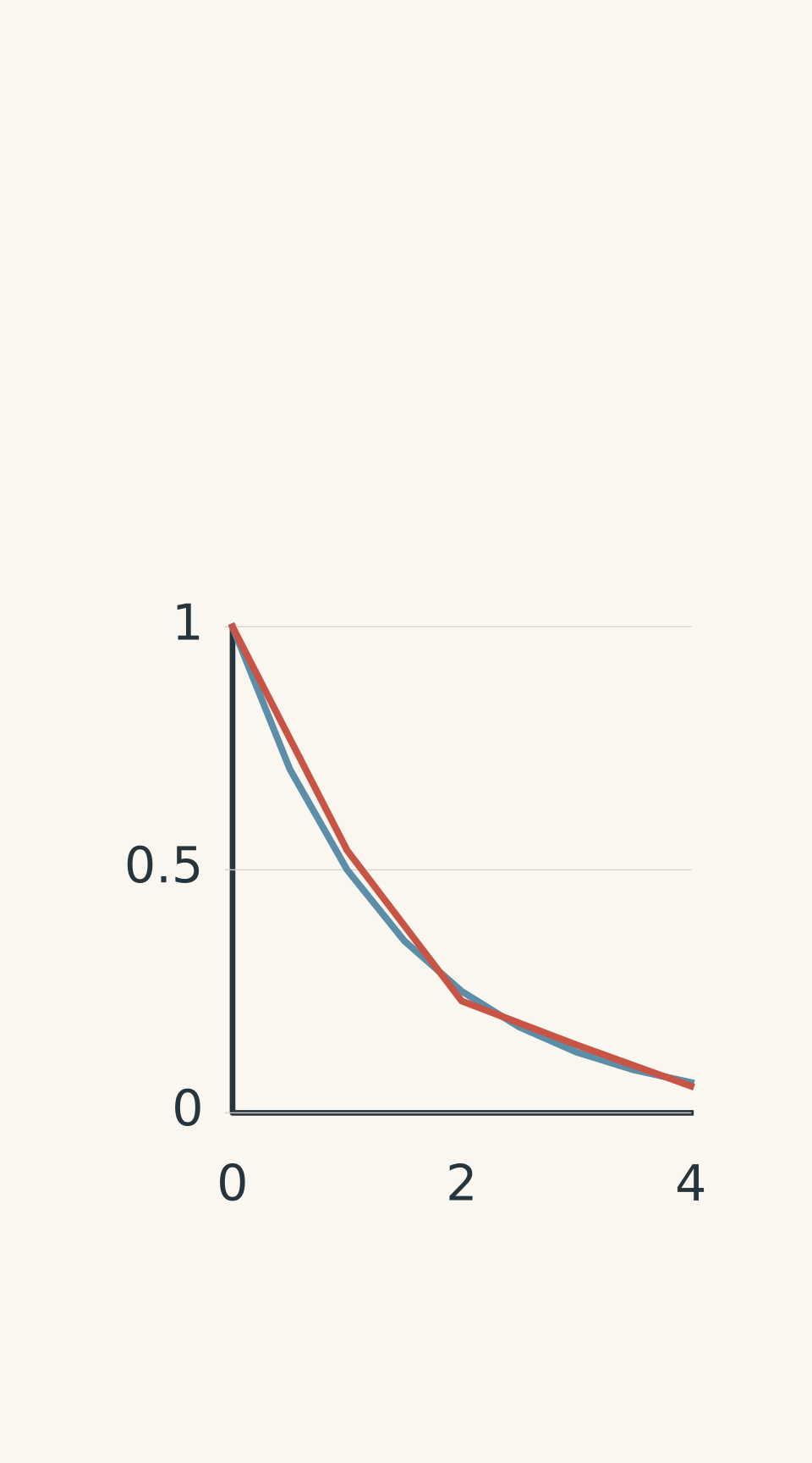
- Expected exponential curve
- Hypothetical measured points
Why the graph curves rather than forming a straight line
During the first half-life, the expected number falls from 800 to 400, a decrease of 400 nuclei.
During the second half-life, it falls from 400 to 200, a decrease of 200 nuclei.
During the third half-life, it falls from 200 to 100, a decrease of 100 nuclei.
The time intervals are equal, but the expected decreases become smaller because fewer undecayed nuclei remain available to decay.
That produces an exponential curve on ordinary linear axes. The curve becomes progressively flatter.
A graph of the expected number remaining approaches zero but does not reach zero at a finite time. A real, finite sample can eventually have no undecayed nuclei left, but the time at which that happens is random.
Do not interpret the curve as a schedule that guarantees when the last nucleus will decay.
Why a large sample follows the curve more closely
Imagine two samples observed after one half-life.
- A sample that begins with 20 nuclei might have 7 remaining. That is 35% of the original sample.
- A sample that begins with 200,000 nuclei might have 99,800 remaining. That is 49.9% of the original sample.
Both are possible outcomes. The first differs substantially from the expected fraction of 50%, while the second is much closer.
Notice that the second sample has a difference of 200 nuclei from its expected count of 100,000. The first differs by only 3 nuclei from its expected count of 10. Yet the larger sample’s fraction is much closer to the prediction.
Same half-life, different statistical fluctuations
| Small sample | 7/20 = 35% Expected: 10 survivors (50%). Difference: 3 nuclei; 15 percentage points below expectation. |
|---|---|
| Large sample | 99,800/200,000 = 49.9% Expected: 100,000 survivors (50%). Difference: 200 nuclei; 0.1 percentage points below expectation. |
This is why radioactive-decay graphs usually look smooth for large samples. The random outcomes of individual nuclei produce relatively small fluctuations in the total fraction remaining.
The expected curve is a statistical prediction, not a claim that every measurement must land exactly on it.
04Check what the detector is actually measuring
There is another trap in half-life questions. A detector’s reading is not necessarily the activity of the radioactive source alone.
A detector may record background radiation as well as radiation from the sample. Its total count rate is
\[ R_{\text{measured}} = R_{\text{source}}+R_{\text{background}} \]
Here, each \(R\) is a count rate, usually measured in counts per minute or counts per second.
Suppose the source initially contributes 500 counts per minute, while the background contributes a constant 30 counts per minute.
The detector reads 530 counts per minute.
After one half-life, the source’s expected count rate falls to 250 counts per minute. The detector now reads
\[ 250+30=280\ \text{counts/min} \]
The total reading has not halved from 530 to 265 because the background has not halved. Only the source’s contribution follows the radioactive-decay law.
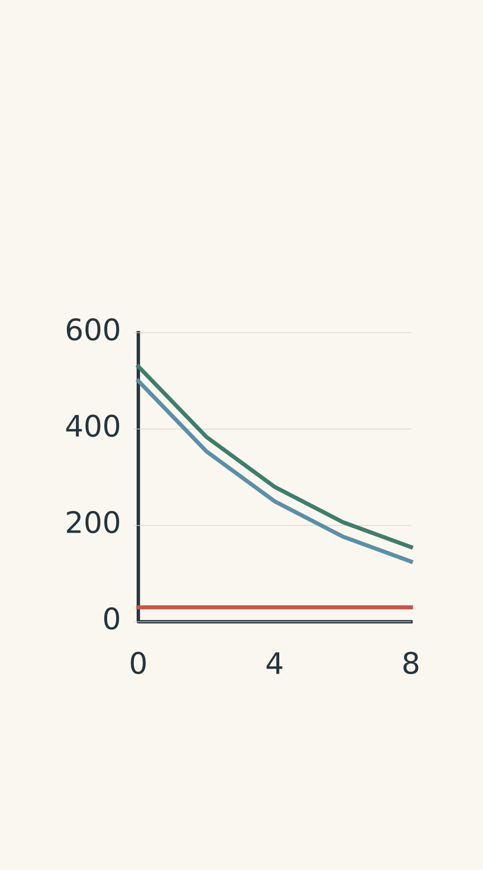
- Source count rate
- Background count rate
- Total measured count rate
When a question gives detector readings, subtract the background before identifying the half-life. If the question later asks for the total detector reading, add the background back.
This is also why experimental count rates can fluctuate around a smooth decay trend. The measured values are counts accumulated over finite intervals, not a perfectly smooth record of every decay.
05A reliable method for half-life questions
Use this decision process under exam conditions.
Step 1: Identify what the question is asking about.
Is it asking when one particular nucleus will decay, or how many nuclei or how much activity a sample is expected to have?
If it asks for an individual nucleus’s exact decay time, the half-life alone cannot provide that answer. If it asks for the probability of decay during the next half-life, the answer is 50%, provided the nucleus is still undecayed at the start of that interval.
Step 2: Identify the initial quantity and the elapsed time.
For a sample, write down \(N_0\), \(t\), and \(T_{1/2}\). If the question concerns activity, use the initial activity \(A_0\) instead of \(N_0\).
Step 3: Calculate the number of half-lives.
\[ n=\frac{t}{T_{1/2}} \]
The quantity \(n\) is the number of half-life intervals elapsed. It can be a fraction, such as 2.5.
Step 4: Apply the decay relationship.
For the expected number of undecayed nuclei,
\[ N_{\text{expected}} = N_0\left(\frac12\right)^n \]
For activity under unchanged conditions,
\[ A_{\text{expected}} = A_0\left(\frac12\right)^n \]
If the question gives raw detector count rates, correct for background first.
Step 5: Interpret the result correctly.
Write “expected number”, “expected activity”, or “approximately” where appropriate. Do not claim that a sample must contain exactly the calculated number of nuclei after a given time.
Worked example: Correcting a half-life prediction
A sample contains 1,600 undecayed nuclei and has a half-life of 5.0 minutes. Estimate the number expected to remain after 15.0 minutes.
A student claims that every nucleus decays after 5.0 minutes, so no nuclei should remain after 15.0 minutes. Identify the error and calculate the correct estimate.
Step 1
The student has treated half-life as the lifetime of each nucleus. It is actually the time over which the expected number of undecayed nuclei halves.
Step 2
\[ n=\frac{15.0\ \text{min}}{5.0\ \text{min}}=3 \]
Three half-lives have elapsed.
Step 3
\[ \begin{aligned} N_{\text{expected}} &=N_0\left(\frac12\right)^n\\ &=1600\left(\frac12\right)^3\\ &=1600\times\frac18\\ &=200\ \text{nuclei} \end{aligned} \]
Step 4
The expected number remaining is 200 nuclei. The sequence is 1,600, 800, 400, then 200.
The student’s prediction of zero is incorrect because three half-lives do not mean that every nucleus has had its full lifetime. The actual count may differ from 200, but the half-life model predicts an expected count of 200.
Worked example: Finding half-life when background counts are present
A detector records 530 counts/min initially, 280 counts/min after 4.0 hours, and 155 counts/min after 8.0 hours. The background count rate is constant at 30 counts/min.
Estimate the source’s half-life and the total detector reading expected after 10.0 hours. Treat the given rates as representative averages.
Step 1
\[ \begin{aligned} R_{\text{source}}(0)&=530-30=500\\ R_{\text{source}}(4.0\text{ h})&=280-30=250\\ R_{\text{source}}(8.0\text{ h})&=155-30=125 \end{aligned} \]
The corrected source count rates are 500, 250, and 125 counts/min.
Step 2
The source count rate halves from 500 to 250 counts/min over 4.0 hours. It halves again from 250 to 125 counts/min over another 4.0 hours.
Therefore,
\[ T_{1/2}=4.0\ \text{h} \]
Step 3
\[ n=\frac{10.0\ \text{h}}{4.0\ \text{h}}=2.5 \]
Apply the half-life relationship:
\[ \begin{aligned} R_{\text{source}}(10.0\text{ h}) &=500\left(\frac12\right)^{2.5}\\ &\approx88.4\ \text{counts/min} \end{aligned} \]
Step 4
\[ \begin{aligned} R_{\text{measured}} &=88.4+30\\ &=118.4\ \text{counts/min} \end{aligned} \]
The expected total detector reading is approximately 118 counts/min, to the nearest whole count per minute.
The important correction is that the source rate halves, not the total reading. Halving the raw initial reading would ignore the constant background contribution.
06The 10-second self-check
Before submitting a half-life answer, ask yourself:
- Am I predicting the behaviour of one nucleus or a sample?
- How many half-lives have elapsed?
- Am I calculating the expected number remaining, rather than the number guaranteed to remain?
- If detector readings are given, have I subtracted the background?
- If an intermediate count is provided, am I predicting from the original sample or from the number actually observed at that time?
That final check becomes particularly important when a question gives you an observed count partway through the decay process.
07Questions and solutions
Question 1
A radioactive sample starts with 3,200 undecayed nuclei. Its half-life is 4.0 minutes. Estimate the expected number of undecayed nuclei remaining after 12.0 minutes.
Solution 1
The expected number remaining is 400 nuclei.
First, calculate the number of half-lives:
\[ n=\frac{12.0\ \text{min}}{4.0\ \text{min}}=3 \]
Then apply the decay relationship:
\[ \begin{aligned} N_{\text{expected}} &=3200\left(\frac12\right)^3\\ &=3200\times\frac18\\ &=400\ \text{nuclei} \end{aligned} \]
Three half-lives reduce the expected number to one-eighth of the initial amount. The answer is an expected count, not a guarantee that exactly 400 nuclei will remain in a particular sample.
Question 2
Ten independent runs of a coin-toss model each begin with 16 coins. The numbers of coins surviving one round are:
\(5,\ 7,\ 8,\ 9,\ 11,\ 6,\ 10,\ 8,\ 7,\ 9\).
(a) Calculate the mean number of survivors.
(b) State the expected number of survivors in a single run.
(c) Explain why the run with 11 survivors does not disprove the model. Would you expect the fraction surviving to vary more or less from run to run if each trial began with 16,000 coins?
Solution 2
(a) The mean is 8 survivors per run.
Add the ten results:
\[ 5+7+8+9+11+6+10+8+7+9=80 \]
Divide by the number of runs:
\[ \text{Mean}=\frac{80}{10}=8 \]
(b) The expected number is also 8 coins.
Each coin has a 50% probability of surviving a round, so the expected number remaining from 16 coins is
\[ 16\times\frac12=8 \]
The mean across the ten runs matches this expectation.
(c) The result of 11 survivors is a random fluctuation, not evidence that the model has failed. The model specifies a 50% survival probability, but does not require exactly eight survivors in every trial.
With 16,000 coins, the fraction surviving would generally fluctuate less around 50%. The absolute number of survivors above or below the expected count could be larger, but that difference would represent a smaller fraction of the much larger sample.
The trap is confusing a probability with a guaranteed outcome in every trial.
Question 3
A detector records 530 counts/min initially, 280 counts/min after 4.0 hours, and 155 counts/min after 8.0 hours. The background count rate is constant at 30 counts/min.
Treat these readings as representative averages.
(a) Estimate the half-life of the source.
(b) Estimate the total detector reading expected after 10.0 hours.
Solution 3
(a) The source’s half-life is 4.0 hours.
Subtract the background from each detector reading:
\[ 530-30=500\ \text{counts/min} \]
\[ 280-30=250\ \text{counts/min} \]
\[ 155-30=125\ \text{counts/min} \]
The source count rate halves every 4.0 hours, so \(T_{1/2}=4.0\ \text{h}\).
(b) The expected total detector reading after 10.0 hours is approximately 118 counts/min.
The elapsed time corresponds to
\[ n=\frac{10.0}{4.0}=2.5 \]
half-lives.
Calculate the expected source rate:
\[ \begin{aligned} R_{\text{source}} &=500\left(\frac12\right)^{2.5}\\ &\approx88.4\ \text{counts/min} \end{aligned} \]
Add the background:
\[ R_{\text{measured}}=88.4+30 \]
\[ R_{\text{measured}}\approx118\ \text{counts/min} \]
The source’s rate follows the half-life relationship. The background remains constant, so the total detector reading does not halve in the same way.
Question 4
Two samples of the same isotope are measured after one half-life.
- Sample S begins with 100 nuclei and has 42 remaining.
- Sample L begins with 1,000,000 nuclei and has 500,120 remaining.
Assume the initial counts and elapsed half-life are known exactly.
(a) Calculate the percentage of nuclei remaining in each sample.
(b) Which sample’s result is closer to the expected fraction?
(c) Does either result prove that the half-life model is incorrect? Explain.
Solution 4
Sample L is much closer to the expected fraction of 50%, and neither observation alone proves that the half-life model is incorrect.
(a) For Sample S,
\[ \frac{42}{100}\times100\%=42\% \]
For Sample L,
\[ \frac{500120}{1000000}\times100\%=50.012\% \]
After one half-life, the expected fraction remaining is 50% for both samples.
(b) Sample L is closer to the expected fraction. Its observed fraction is 50.012%, compared with Sample S’s 42%.
(c) Neither result contradicts the decay model. Radioactive decay is statistical, so an individual sample can differ from its expected count. Such deviations are generally more noticeable as a fraction of the total in small samples.
The tempting mistake is to assume that the half-life guarantees exactly half the nuclei will survive every interval. It predicts the statistical behaviour of the sample, not an exact count in every measurement.
Question 5
Two independent samples of the same isotope each begin with 800 undecayed nuclei. The half-life is 10.0 minutes.
At \(t=20.0\) minutes, Sample A has 210 nuclei remaining, while Sample B has 190 nuclei remaining. Treat these as exact counts, with no detector counting error. Assume no new nuclei are produced and that decays are independent.
A student argues that both samples must contain 100 nuclei at \(t=30.0\) minutes because three half-lives have elapsed. Another student predicts expected counts of 105 for Sample A and 95 for Sample B.
(a) Before knowing the actual counts at 20.0 minutes, what number of nuclei would be expected in each sample at 30.0 minutes?
(b) Once the actual counts at 20.0 minutes are known, calculate the expected number remaining at 30.0 minutes for each sample.
(c) A nucleus is selected from Sample A’s 210 survivors at 20.0 minutes. What is the probability that it decays during the next 10.0 minutes? Does its survival for the first 20.0 minutes change that probability?
(d) Reconcile the two predictions for the sample counts. Explain why neither prediction implies that half-life is a countdown for individual nuclei.
Solution 5
Before the intermediate counts are known, both samples have an expected count of 100 nuclei at 30.0 minutes. Once their actual counts at 20.0 minutes are known, the conditional expected counts become 105 for Sample A and 95 for Sample B. The selected nucleus has a 50% probability of decaying during the next 10.0 minutes.
The key is that these are answers to different questions.
(a) Expected counts before the 20-minute observations
Three half-lives have elapsed by \(t=30.0\) minutes:
\[ n=\frac{30.0\ \text{min}}{10.0\ \text{min}}=3 \]
For either sample,
\[ \begin{aligned} N_{\text{expected}} &=800\left(\frac12\right)^3\\ &=800\times\frac18\\ &=100\ \text{nuclei} \end{aligned} \]
Before observing the intermediate counts, the expected number at 30.0 minutes is 100 for each sample.
This is an average prediction based on the initial count. It does not guarantee that either sample will contain exactly 100 nuclei.
(b) Expected counts after observing the 20-minute results
At 20.0 minutes, Sample A actually has 210 nuclei remaining. One more half-life is 10.0 minutes, so its conditional expected count is
\[ N_{\text{A, expected}}=210\times\frac12=105 \]
Sample B actually has 190 nuclei remaining, giving
\[ N_{\text{B, expected}}=190\times\frac12=95 \]
These are the correct expected counts when we use the observed state of each sample at 20.0 minutes as the starting point for the next interval.
(c) Probability that the selected nucleus decays
The probability is 50%.
The selected nucleus has survived for 20.0 minutes, but that does not change its probability of decaying during the next 10.0 minutes. For an undecayed nucleus, the probability of decay during an interval equal to one half-life is 50%, regardless of how long it has already survived.
The nucleus is not overdue. It may decay during the next interval, or it may survive it.
(d) Why both sample predictions can be correct
The predictions of 100 and 105 for Sample A answer different questions.
- The value of 100 is the expected count at 30.0 minutes when predicting from the original sample of 800 nuclei, without knowing the actual count at 20.0 minutes.
- The value of 105 is the expected count at 30.0 minutes after observing that 210 nuclei actually remain at 20.0 minutes.
The same distinction applies to Sample B: 100 is the original prediction, while 95 is the conditional prediction based on its observed count.
There is no contradiction. The observed counts at 20.0 minutes differ from the expected count of 200. Once that information is known, it is sensible to update the prediction for the next interval.
The crucial distinction is that an expected count is not an exact future count. Even after using the observed intermediate count, the number remaining at 30.0 minutes may differ from 105 or 95 because the next set of decays is also random.
This is the deeper meaning of half-life: the same decay law governs the sample throughout, but the exact outcomes of individual decays remain unpredictable.
The next time you interpret a radioactive-decay graph, identify what the vertical axis measures first: expected nuclei, source activity, or total detector count rate. Then check whether you are predicting from the original sample or from an observed intermediate count. Those decisions determine which calculation is appropriate and prevent a correct formula from producing a misleading conclusion.