
Why the Smallest Ksp Does Not Always Mean the Least Soluble Salt
A smaller Ksp does not always mean a salt is less soluble. Learn how dissolution stoichiometry changes the relationship between Ksp and molar solubility, work through HSC Chemistry calculations, and convert solubility into grams per litre.
You compare two solubility product values at 25 °C: \(K_{sp}(\ce{AgCl})=1.8\times10^{-10}\) and \(K_{sp}(\ce{CaF2})=3.9\times10^{-11}\). You circle \(\ce{CaF2}\) as the less soluble salt because its \(K_{sp}\) is smaller. That looks reasonable, but it’s wrong. In pure water, \(\ce{CaF2}\) has a higher molar solubility than \(\ce{AgCl}\). The problem isn’t your arithmetic. It’s that you’re treating \(K_{sp}\) as if it were a direct measurement of solubility.
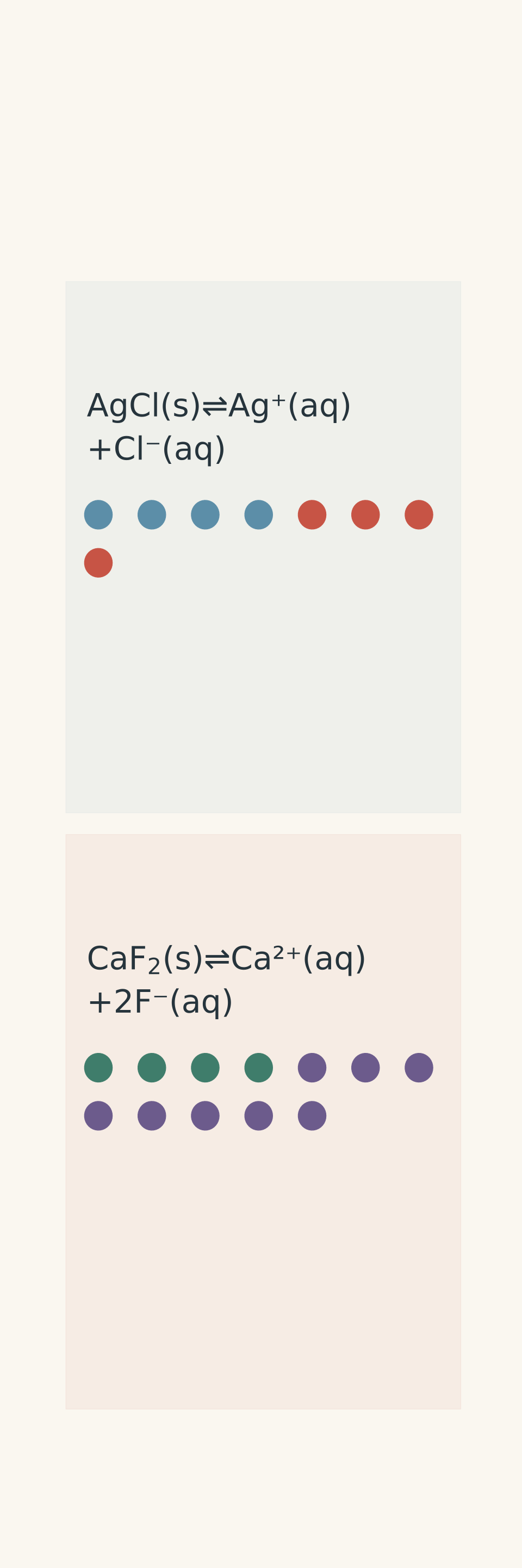
- Ag⁺
- Cl⁻
- Ca²⁺
- F⁻
01The mistake: treating \(K_{sp}\) like a solubility score
The solubility product, \(K_{sp}\), is an equilibrium constant. It describes the equilibrium concentrations of dissolved ions in a saturated solution.
It does not tell you the molar solubility directly.
The difference becomes clear when you look at the balanced dissolution equations. Consider these two salts.
For silver chloride:
\[ \ce{AgCl(s) <=> Ag+(aq) + Cl-(aq)} \]
For calcium fluoride:
\[ \ce{CaF2(s) <=> Ca^2+(aq) + 2F-(aq)} \]
Notice the difference. One mole of dissolved \(\ce{AgCl}\) produces one mole of \(\mathrm{Ag}^{+}\) and one mole of \(\mathrm{Cl}^{-}\). One mole of dissolved \(\ce{CaF2}\) produces one mole of \(\mathrm{Ca}^{2+}\) and two moles of \(\mathrm{F}^{-}\).
That difference changes the mathematical relationship between the amount dissolved and the equilibrium concentrations.
Start with molar solubility
Let \(s\) represent the molar solubility of a salt: the number of moles of formula units that dissolve per litre of solution to produce a saturated solution.
Its units are \(\mathrm{mol\,L^{-1}}\).
Assume the salt dissolves in pure water, with no other source of its ions, and that we can use concentrations in place of activities. These are the usual simplifying assumptions for this type of HSC calculation.
For \(\ce{AgCl}\), if \(s\) mol L\(^{-1}\) dissolves, the equation produces equal concentrations of both ions:
\[ [\mathrm{Ag}^{+}]=s \]
\[ [\mathrm{Cl}^{-}]=s \]
For \(\ce{CaF2}\), the calcium-to-fluoride ratio is \(1:2\):
\[ [\mathrm{Ca}^{2+}]=s \]
\[ [\mathrm{F}^{-}]=2s \]
The coefficient of an ion in the balanced equation determines its concentration relative to \(s\). That coefficient must be accounted for before you substitute into the \(K_{sp}\) expression.
From dissolution stoichiometry to Ksp
| Silver chloride (AgCl) | AgCl(s) ⇌ Ag⁺(aq) + Cl⁻(aq) Dissolution ratio 1:1 → [Ag⁺] = s; [Cl⁻] = s. Substitute into Ksp → Ksp = [Ag⁺][Cl⁻] = s × s = s². |
|---|---|
| Calcium fluoride (CaF₂) | CaF₂(s) ⇌ Ca²⁺(aq) + 2F⁻(aq) Dissolution ratio 1:2 → [Ca²⁺] = s; [F⁻] = 2s. Coefficient 2 gives [F⁻] = 2s; exponent 2 squares it → Ksp = [Ca²⁺][F⁻]² = s(2s)² = 4s³. |
Derive the two \(K_{sp}\) expressions
For silver chloride, the solid is omitted from the equilibrium expression:
\[ K_{sp}=[\mathrm{Ag}^{+}][\mathrm{Cl}^{-}] \]
Substitute the equilibrium concentrations:
\[ K_{sp}=s\times s \]
Therefore,
\[ \boxed{K_{sp}=s^2} \]
For calcium fluoride, the fluoride concentration is \(2s\), and its concentration is squared in the equilibrium expression:
\[ K_{sp}=[\mathrm{Ca}^{2+}][\mathrm{F}^{-}]^2 \]
Substitute:
\[ \begin{aligned} K_{sp}&=s(2s)^2\\ &=4s^3 \end{aligned} \]
Therefore,
\[ \boxed{K_{sp}=4s^3} \]
This is the crucial difference. The first salt has a squared relationship between \(K_{sp}\) and \(s\). The second has a cubed relationship, including a factor of four.
You cannot rank their solubilities by comparing the two \(K_{sp}\) numbers alone.
If you need a refresher on writing equilibrium expressions, see tutorgum’s HSC Chemistry Module 5 Equilibrium: Complete Topic Summary.
02Worked examples: from \(K_{sp}\) to actual solubility
Worked example: Find the solubility of AgCl
At 25 °C, silver chloride has \(K_{sp}=1.8\times10^{-10}\). Calculate its molar solubility in pure water and convert the result to grams per litre. The molar mass of \(\ce{AgCl}\) is \(143.32\ \mathrm{g\,mol^{-1}}\).
Step 1
\[ \ce{AgCl(s) <=> Ag+(aq) + Cl-(aq)} \]
One mole of \(\ce{AgCl}\) produces one mole of each ion. Therefore,
\[ [\mathrm{Ag}^{+}]=s,\qquad [\mathrm{Cl}^{-}]=s \]
Step 2
\[ K_{sp}=[\mathrm{Ag}^{+}][\mathrm{Cl}^{-}]=s^2 \]
Step 3
\[ \begin{aligned} s^2&=1.8\times10^{-10}\\ s&=\sqrt{1.8\times10^{-10}}\\ s&=1.34\times10^{-5}\ \mathrm{mol\,L^{-1}} \end{aligned} \]
The molar solubility is \(1.34\times10^{-5}\ \mathrm{mol\,L^{-1}}\).
Step 4
Molar solubility tells you how many moles dissolve per litre. To find the mass that dissolves per litre, multiply by the molar mass.
\[ \begin{aligned} \text{Mass solubility} &=s\times M\\ &=(1.34\times10^{-5})(143.32)\\ &=1.92\times10^{-3}\ \mathrm{g\,L^{-1}} \end{aligned} \]
Here, \(M\) is the molar mass in \(\mathrm{g\,mol^{-1}}\). The mole units cancel, leaving grams per litre.
Converting grams to milligrams gives:
\[ \boxed{1.92\ \mathrm{mg\,L^{-1}}} \]
A saturated solution contains approximately \(1.92\) mg of dissolved \(\ce{AgCl}\) per litre under these conditions.
From Ksp to mass solubility: AgCl
- Start with Ksp
AgCl(s) ⇌ Ag⁺(aq) + Cl⁻(aq)
Ksp = s² = 1.8 × 10⁻¹⁰
Each ion concentration equals s.
- Calculate molar solubility
s = √(1.8 × 10⁻¹⁰)
s = 1.34 × 10⁻⁵ mol L⁻¹
This is the amount in moles of AgCl dissolved per litre.
- Convert to mass solubility
(1.34 × 10⁻⁵ mol L⁻¹) × (143.32 g mol⁻¹)
Molar mass of AgCl = 143.32 g mol⁻¹.
Mass solubility = 1.92 × 10⁻³ g L⁻¹ = 1.92 mg L⁻¹.
Worked example: Find the solubility of CaF2
At 25 °C, calcium fluoride has \(K_{sp}=3.9\times10^{-11}\). Calculate its molar solubility in pure water and convert the result to grams per litre. The molar mass of \(\ce{CaF2}\) is \(78.07\ \mathrm{g\,mol^{-1}}\). Compare its solubility with that of \(\ce{AgCl}\).
Step 1
\[ \ce{CaF2(s) <=> Ca^2+(aq) + 2F-(aq)} \]
Step 2
For every mole of \(\ce{CaF2}\) that dissolves, one mole of \(\mathrm{Ca}^{2+}\) and two moles of \(\mathrm{F}^{-}\) enter the solution.
Therefore,
\[ [\mathrm{Ca}^{2+}]=s,\qquad [\mathrm{F}^{-}]=2s \]
Step 3
\[ \begin{aligned} K_{sp}&=[\mathrm{Ca}^{2+}][\mathrm{F}^{-}]^2\\ &=s(2s)^2\\ &=4s^3 \end{aligned} \]
Step 4
\[ \begin{aligned} 3.9\times10^{-11}&=4s^3\\ s^3&=\frac{3.9\times10^{-11}}{4}\\ s&=\sqrt[3]{9.75\times10^{-12}}\\ s&=2.14\times10^{-4}\ \mathrm{mol\,L^{-1}} \end{aligned} \]
The molar solubility of \(\ce{CaF2}\) is \(2.14\times10^{-4}\ \mathrm{mol\,L^{-1}}\).
Step 5
\[ \begin{aligned} \text{Mass solubility} &=s\times M\\ &=(2.14\times10^{-4})(78.07)\\ &=1.67\times10^{-2}\ \mathrm{g\,L^{-1}}\\ &=16.7\ \mathrm{mg\,L^{-1}} \end{aligned} \]
Step 6
| Property | AgCl | CaF2 |
|---|---|---|
| \(K_{sp}\) | \(1.8\times10^{-10}\) | \(3.9\times10^{-11}\) |
| Molar solubility (\(\mathrm{mol\,L^{-1}}\)) | \(1.34\times10^{-5}\) | \(2.14\times10^{-4}\) |
| Mass solubility (\(\mathrm{mg\,L^{-1}}\)) | 1.92 | 16.7 |
Although \(\ce{CaF2}\) has the smaller \(K_{sp}\), it has approximately 16 times the molar solubility of \(\ce{AgCl}\) and about 8.7 times its mass solubility.
The tempting mistake was to assume that a smaller \(K_{sp}\) must correspond to a smaller \(s\). That would only be a valid shortcut if the salts had the same mathematical relationship between \(K_{sp}\) and \(s\).
Smaller Ksp, greater solubility
| Panel 1 — Solubility product, Ksp | AgCl versus CaF₂ AgCl: 1.8 × 10⁻¹⁰ CaF₂: 3.9 × 10⁻¹¹ — smaller Ksp. |
|---|---|
| Panel 2 — Molar solubility | mol L⁻¹ AgCl: 1.34 × 10⁻⁵ mol L⁻¹ CaF₂: 2.14 × 10⁻⁴ mol L⁻¹ — about 16 times greater. |
| Panel 3 — Mass solubility | mg L⁻¹ AgCl: 1.92 mg L⁻¹ CaF₂: 16.7 mg L⁻¹ — about 8.7 times greater. |
03Why memorised shortcuts break
There are three related mistakes to watch for.
Mistake 1: Assuming the smallest \(K_{sp}\) means the least soluble salt
The shortcut fails when salts have different dissolution stoichiometries.
| Dissolution type | Relationship in pure water | Solubility expression |
|---|---|---|
| \(AB(s)\rightleftharpoons A^+(aq)+B^-(aq)\) | \(K_{sp}=s^2\) | \(s=\sqrt{K_{sp}}\) |
| \(AB_2(s)\rightleftharpoons A^{2+}(aq)+2B^-(aq)\) | \(K_{sp}=4s^3\) | \(s=\sqrt[3]{K_{sp}/4}\) |
These are examples of the general rule: derive the expression from the balanced equation, then solve for \(s\).
There is a situation in which the shortcut works. If two salts have the same dissolution stoichiometry, are compared at the same temperature, and are dissolved under the same assumptions, their \(K_{sp}\) values have the same mathematical relationship to molar solubility. For two 1:1 salts, for example, a lower \(K_{sp}\) means a lower molar solubility.
The problem is comparing salts with different stoichiometries as though they followed the same equation.
Mistake 2: Confusing molar solubility with mass solubility
Molar solubility measures moles dissolved per litre. Mass solubility measures grams dissolved per litre.
The conversion is:
\[ \boxed{\text{Mass solubility}=s\times M} \]
A salt with a higher molar solubility does not necessarily have a higher mass solubility. Its molar mass also matters.
For example, imagine that Salt A dissolves to \(0.0020\ \mathrm{mol\,L^{-1}}\) and has a molar mass of \(300\ \mathrm{g\,mol^{-1}}\). Its mass solubility is \(0.60\ \mathrm{g\,L^{-1}}\).
Salt B might dissolve to \(0.010\ \mathrm{mol\,L^{-1}}\) but have a molar mass of only \(50\ \mathrm{g\,mol^{-1}}\). Its mass solubility is \(0.50\ \mathrm{g\,L^{-1}}\).
Salt B dissolves more formula units per litre, but Salt A dissolves more grams per litre. Neither statement contradicts the other. They describe different quantities.
Mistake 3: Assuming the solution contains only ions produced by the dissolving salt
So far, we’ve assumed pure water. That assumption matters.
Suppose you dissolve \(\ce{CaF2}\) in a solution that already contains fluoride ions, such as aqueous \(\ce{NaF}\). The fluoride concentration is no longer simply \(2s\). It includes fluoride already present in the solution:
\[ [\mathrm{F}^{-}]=[\mathrm{F}^{-}]_{\text{initial}}+2s \]
The same \(K_{sp}\) expression still applies, but the equilibrium concentrations are different. The existing fluoride ions suppress further dissolution of \(\ce{CaF2}\). This is the common-ion effect.
At the same temperature, \(K_{sp}\) remains constant in the ideal concentration model used here. The solubility changes because the other ion concentrations have changed.
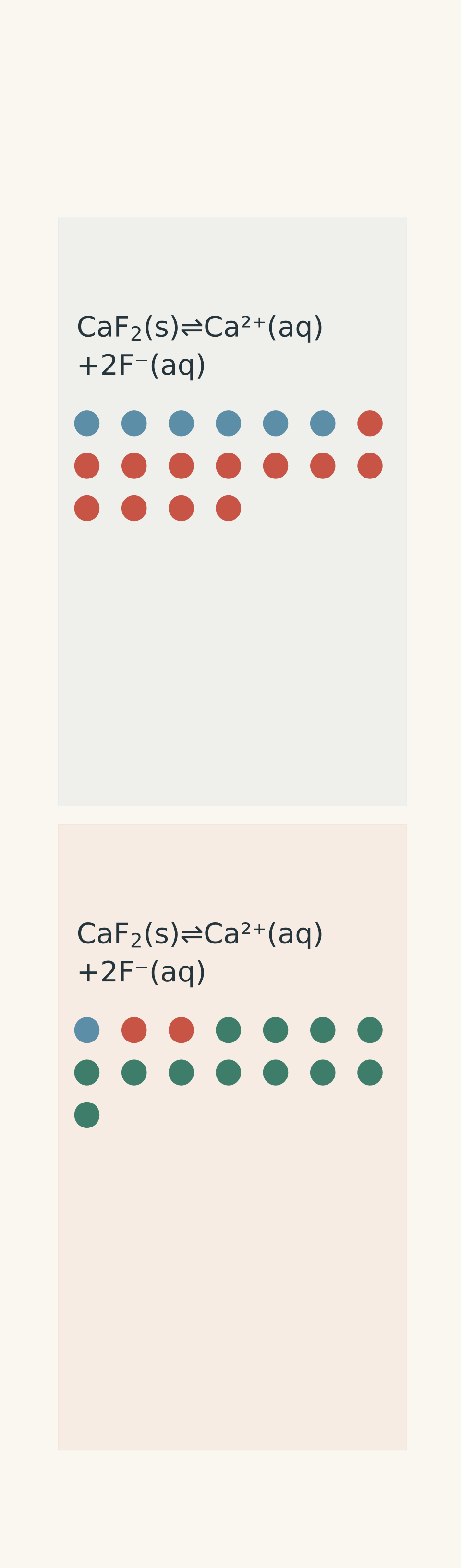
- Ca²⁺ from CaF₂
- F⁻ from CaF₂
- F⁻ supplied by NaF
04A method you can reuse in an exam
When a question asks you to compare solubilities, follow this sequence rather than reaching for a shortcut.
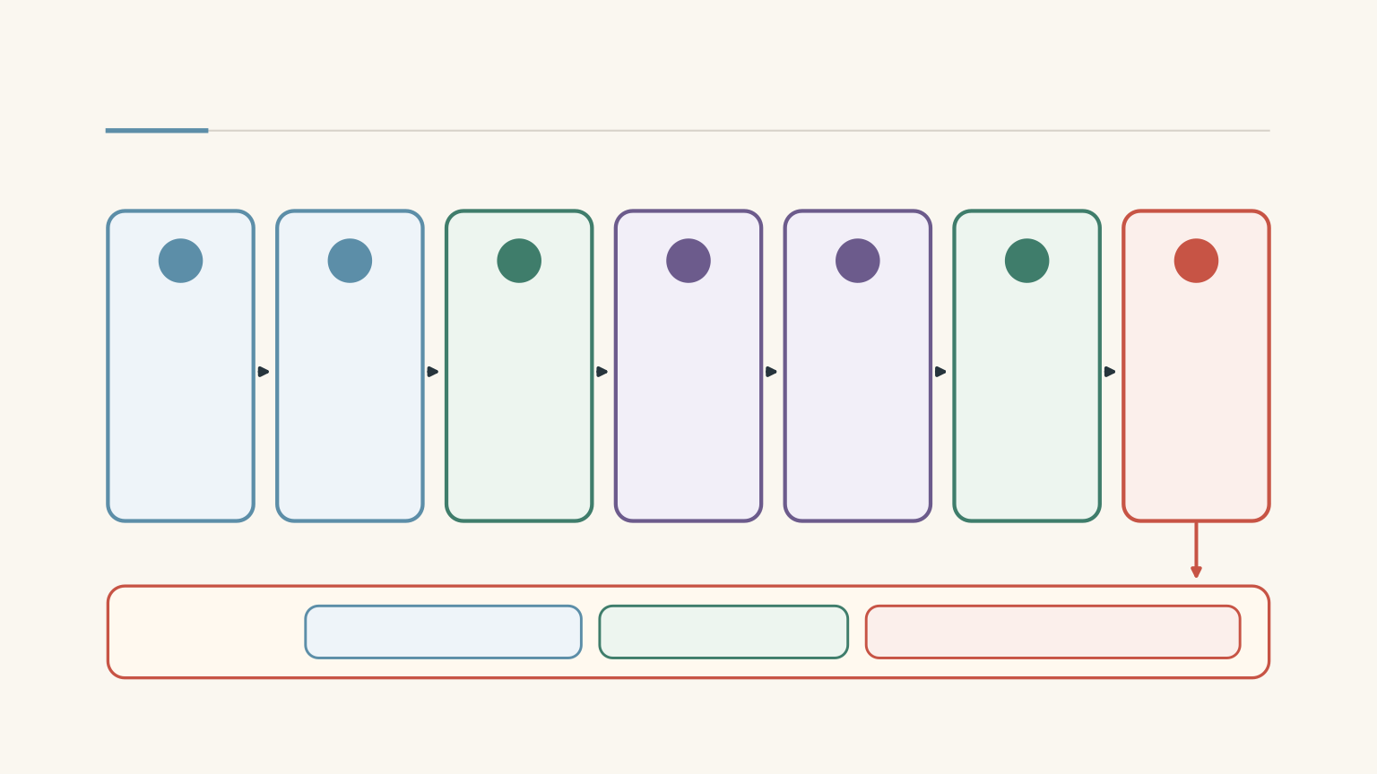
Step 1: Write the balanced dissolution equation.
Identify the number and charge of each ion produced by one formula unit of the salt.
Step 2: Define \(s\).
Let \(s\) be the molar solubility in \(\mathrm{mol\,L^{-1}}\).
Step 3: Convert the stoichiometric coefficients into concentrations.
If the equation produces two moles of an ion for every mole of salt dissolved, its concentration contribution is \(2s\), not \(s\).
Step 4: Write the \(K_{sp}\) expression.
Use the equilibrium ion concentrations, raising each concentration to the power of its coefficient in the balanced equation. Pure solids are omitted.
Step 5: Solve for \(s\).
Use the appropriate root or rearrangement. Keep the units as \(\mathrm{mol\,L^{-1}}\).
Step 6: Convert only if needed.
If the question asks for grams per litre, multiply \(s\) by the molar mass. If it asks which salt is more soluble, specify whether you’re comparing molar solubility, mass solubility, or the total concentration of dissolved ions.
A quick exam self-check
Before you move on from a solubility calculation, ask yourself:
- Have I balanced the dissolution equation?
- Have I used the stoichiometric coefficients to determine the ion concentrations?
- Have I applied the powers in the \(K_{sp}\) expression correctly?
- Is the solution pure water, or is a common ion already present?
- Am I comparing molar solubility or mass solubility?
- Have I converted to grams per litre only after finding \(s\)?
If you can answer all six, you’re much less likely to lose marks to a correct-looking but invalid comparison.
05Questions and solutions
Question 1
At 25 °C, silver bromide has \(K_{sp}=5.0\times10^{-13}\). Write its dissolution equation and calculate its molar solubility in pure water. Assume no complex-ion formation.
Solution 1
The molar solubility is \(7.1\times10^{-7}\ \mathrm{mol\,L^{-1}}\). Because silver bromide dissolves in a 1:1 ratio, its \(K_{sp}\) expression is \(s^2\).
The dissolution equation is:
\[ \ce{AgBr(s) <=> Ag+(aq) + Br-(aq)} \]
Let \(s\) be the molar solubility. Then:
\[ [\mathrm{Ag}^{+}]=s,\qquad [\mathrm{Br}^{-}]=s \]
Therefore,
\[ \begin{aligned} K_{sp}&=[\mathrm{Ag}^{+}][\mathrm{Br}^{-}]\\ &=s^2\\ 5.0\times10^{-13}&=s^2\\ s&=\sqrt{5.0\times10^{-13}}\\ &=7.1\times10^{-7}\ \mathrm{mol\,L^{-1}} \end{aligned} \]
The square root is appropriate because each formula unit produces one ion of each type. Using a cube root here would incorrectly assume a different dissolution stoichiometry.
Question 2
At 25 °C, strontium fluoride has \(K_{sp}=2.6\times10^{-9}\). Calculate:
(a) its molar solubility in pure water;
(b) the equilibrium fluoride-ion concentration;
(c) its mass solubility in \(\mathrm{g\,L^{-1}}\).
The molar mass of \(\ce{SrF2}\) is \(125.62\ \mathrm{g\,mol^{-1}}\).
Solution 2
The molar solubility is \(8.7\times10^{-4}\ \mathrm{mol\,L^{-1}}\), the fluoride-ion concentration is \(1.7\times10^{-3}\ \mathrm{mol\,L^{-1}}\), and the mass solubility is approximately \(0.11\ \mathrm{g\,L^{-1}}\).
The key is to use the 1:2 dissolution ratio before calculating any of these quantities.
The dissolution equation is:
\[ \ce{SrF2(s) <=> Sr^2+(aq) + 2F-(aq)} \]
Step 1: Express the ion concentrations in terms of \(s\).
\[ [\mathrm{Sr}^{2+}]=s,\qquad [\mathrm{F}^{-}]=2s \]
Step 2: Write the \(K_{sp}\) expression.
\[ \begin{aligned} K_{sp}&=[\mathrm{Sr}^{2+}][\mathrm{F}^{-}]^2\\ &=s(2s)^2\\ &=4s^3 \end{aligned} \]
Step 3: Calculate the molar solubility.
\[ \begin{aligned} 2.6\times10^{-9}&=4s^3\\ s&=\sqrt[3]{\frac{2.6\times10^{-9}}{4}}\\ &=\sqrt[3]{6.5\times10^{-10}}\\ &=8.7\times10^{-4}\ \mathrm{mol\,L^{-1}} \end{aligned} \]
Step 4: Calculate the fluoride-ion concentration.
Each mole of dissolved \(\ce{SrF2}\) produces two moles of fluoride ions:
\[ \begin{aligned} [\mathrm{F}^{-}]&=2s\\ &=2(8.7\times10^{-4})\\ &=1.7\times10^{-3}\ \mathrm{mol\,L^{-1}} \end{aligned} \]
Step 5: Convert to mass solubility.
\[ \begin{aligned} \text{Mass solubility} &=s\times M\\ &=(8.7\times10^{-4})(125.62)\\ &\approx0.11\ \mathrm{g\,L^{-1}} \end{aligned} \]
The three answers describe different quantities. Molar solubility counts dissolved formula units, fluoride concentration counts one particular ion, and mass solubility measures the mass of salt dissolved per litre.
Question 3
Two hypothetical salts dissolve in pure water at the same temperature.
- Salt A dissolves in a 1:1 ratio and has \(K_{sp}=4.0\times10^{-8}\).
- Salt B dissolves to produce one cation and two anions per formula unit, and has \(K_{sp}=1.0\times10^{-10}\).
A student concludes that Salt B must be less soluble because its \(K_{sp}\) is smaller. Calculate the molar solubility of each salt and assess the student’s conclusion.
Solution 3
Salt B is actually more soluble in molar terms: its molar solubility is approximately \(2.9\times10^{-4}\ \mathrm{mol\,L^{-1}}\), compared with \(2.0\times10^{-4}\ \mathrm{mol\,L^{-1}}\) for Salt A. The student’s mistake is comparing the raw \(K_{sp}\) values without accounting for the different dissolution ratios.
Step 1: Calculate the molar solubility of Salt A.
For a 1:1 salt:
\[ K_{sp}=s^2 \]
Therefore,
\[ \begin{aligned} s_A&=\sqrt{4.0\times10^{-8}}\\ &=2.0\times10^{-4}\ \mathrm{mol\,L^{-1}} \end{aligned} \]
Step 2: Derive the expression for Salt B.
Its dissolution equation has the general form:
\[ \ce{CD2(s) <=> C^2+(aq) + 2D-(aq)} \]
Therefore,
\[ K_{sp}=s(2s)^2=4s^3 \]
Step 3: Calculate the molar solubility of Salt B.
\[ \begin{aligned} s_B&=\sqrt[3]{\frac{1.0\times10^{-10}}{4}}\\ &=\sqrt[3]{2.5\times10^{-11}}\\ &=2.9\times10^{-4}\ \mathrm{mol\,L^{-1}} \end{aligned} \]
Salt B has the smaller \(K_{sp}\), yet the larger molar solubility. The reason is that its \(K_{sp}\) depends on the cube of \(s\), whereas Salt A’s depends on the square of \(s\).
The exact comparison requires solving both expressions. The size of the \(K_{sp}\) values alone does not determine the ranking when the stoichiometries differ.
Question 4
At 25 °C, calcium fluoride has \(K_{sp}=3.9\times10^{-11}\). Estimate its molar solubility in \(0.0100\ \mathrm{mol\,L^{-1}}\) aqueous \(\ce{NaF}\).
Assume \(\ce{NaF}\) dissociates completely, concentration-based equilibrium expressions are appropriate, and the additional fluoride produced by dissolving \(\ce{CaF2}\) is negligible compared with the fluoride already present. Compare your result with the molar solubility in pure water and explain why \(K_{sp}\) does not change.
Solution 4
The molar solubility in \(0.0100\ \mathrm{mol\,L^{-1}}\) \(\ce{NaF}\) is approximately \(3.9\times10^{-7}\ \mathrm{mol\,L^{-1}}\). This is about 550 times lower than the solubility in pure water because the solution already contains fluoride ions.
Step 1: Start with the correct equilibrium expression.
\[ K_{sp}=[\mathrm{Ca}^{2+}][\mathrm{F}^{-}]^2 \]
Let \(s\) be the molar solubility of \(\ce{CaF2}\). Then:
\[ [\mathrm{Ca}^{2+}]=s \]
The total fluoride concentration is initially:
\[ [\mathrm{F}^{-}]=0.0100+2s \]
Step 2: Apply the stated approximation.
Because \(2s\) is negligible compared with \(0.0100\ \mathrm{mol\,L^{-1}}\),
\[ [\mathrm{F}^{-}]\approx0.0100\ \mathrm{mol\,L^{-1}} \]
Substitute into the \(K_{sp}\) expression:
\[ \begin{aligned} 3.9\times10^{-11}&=s(0.0100)^2\\ s&=\frac{3.9\times10^{-11}}{1.00\times10^{-4}}\\ &=3.9\times10^{-7}\ \mathrm{mol\,L^{-1}} \end{aligned} \]
Step 3: Compare with pure water.
From the earlier calculation, the molar solubility in pure water is:
\[ s_{\text{pure}}=2.14\times10^{-4}\ \mathrm{mol\,L^{-1}} \]
The ratio is:
\[ \begin{aligned} \frac{s_{\text{pure}}}{s_{\ce{NaF}}} &=\frac{2.14\times10^{-4}}{3.9\times10^{-7}}\\ &\approx550 \end{aligned} \]
The solubility is therefore about 550 times lower in the sodium fluoride solution.
The tempting mistake is to assume that \(K_{sp}\) changes when the solution changes. At the same temperature, the equilibrium constant remains fixed in this model. The common ion changes the equilibrium concentrations needed to satisfy that constant, suppressing further dissolution.
Question 5
Two hypothetical salts have the same numerical \(K_{sp}\) at 25 °C:
- Salt A has formula \(AB\), dissolving as \(A^+ + B^-\), and a molar mass of \(300\ \mathrm{g\,mol^{-1}}\).
- Salt C has formula \(CD_2\), dissolving as \(C^{2+} + 2D^-\), and a molar mass of \(50\ \mathrm{g\,mol^{-1}}\).
Both salts have \(K_{sp}=4.0\times10^{-6}\).
Separate \(0.100\ \mathrm{g}\) samples of each salt are added to separate \(100.0\ \mathrm{mL}\) portions of pure water. After equilibrium is reached, undissolved solid remains in both containers.
Assume the solution volumes remain \(100.0\ \mathrm{mL}\), the concentration-based equilibrium model is valid, and no side reactions occur.
For each salt:
(a) Calculate its molar solubility.
(b) Calculate the mass that dissolves and the mass that remains undissolved.
(c) Calculate the total dissolved ion concentration, defined as the sum of the equilibrium concentrations of all dissolved ions.
(d) Explain whether Salt A or Salt C is less soluble.
Solution 5
Salt A dissolves more mass: \(0.0600\ \mathrm{g}\), compared with \(0.0500\ \mathrm{g}\) for Salt C. However, Salt C dissolves five times as many moles of formula units and produces 7.5 times the total concentration of dissolved ions. Neither salt is simply “less soluble” without specifying which measure of solubility is being compared.
The important constraint is that equal \(K_{sp}\) values do not imply equal molar solubilities when the dissolution stoichiometries differ. Molar mass then creates another difference between molar and mass solubility.
Step 1: Calculate the molar solubility of Salt A.
Its dissolution equation is:
\[ \ce{AB(s) <=> A+(aq) + B-(aq)} \]
Therefore,
\[ K_{sp}=s_A^2 \]
Substitute the given value:
\[ \begin{aligned} s_A&=\sqrt{4.0\times10^{-6}}\\ &=2.0\times10^{-3}\ \mathrm{mol\,L^{-1}} \end{aligned} \]
Step 2: Calculate the mass solubility of Salt A.
\[ \begin{aligned} \text{Mass solubility}_A &=s_A\times M_A\\ &=(2.0\times10^{-3})(300)\\ &=0.600\ \mathrm{g\,L^{-1}} \end{aligned} \]
In \(0.1000\ \mathrm{L}\), the maximum mass that can dissolve at saturation is:
\[ \begin{aligned} m_{\text{dissolved},A} &=(0.600)(0.1000)\\ &=0.0600\ \mathrm{g} \end{aligned} \]
The initial sample was \(0.100\ \mathrm{g}\), so the mass remaining is:
\[ \begin{aligned} m_{\text{remaining},A} &=0.100-0.0600\\ &=0.0400\ \mathrm{g} \end{aligned} \]
Step 3: Calculate the molar solubility of Salt C.
Its dissolution equation is:
\[ \ce{CD2(s) <=> C^2+(aq) + 2D-(aq)} \]
The equilibrium concentrations are:
\[ [\mathrm{C}^{2+}]=s_C,\qquad [\mathrm{D}^{-}]=2s_C \]
Therefore,
\[ K_{sp}=s_C(2s_C)^2=4s_C^3 \]
Substitute the given value:
\[ \begin{aligned} s_C&=\sqrt[3]{\frac{4.0\times10^{-6}}{4}}\\ &=\sqrt[3]{1.0\times10^{-6}}\\ &=1.00\times10^{-2}\ \mathrm{mol\,L^{-1}} \end{aligned} \]
Salt C has five times the molar solubility of Salt A:
\[ \frac{s_C}{s_A} =\frac{1.00\times10^{-2}}{2.0\times10^{-3}} =5.0 \]
Step 4: Calculate the mass dissolved and the mass remaining for Salt C.
\[ \begin{aligned} \text{Mass solubility}_C &=s_C\times M_C\\ &=(1.00\times10^{-2})(50)\\ &=0.500\ \mathrm{g\,L^{-1}} \end{aligned} \]
In \(0.1000\ \mathrm{L}\):
\[ \begin{aligned} m_{\text{dissolved},C} &=(0.500)(0.1000)\\ &=0.0500\ \mathrm{g} \end{aligned} \]
The mass remaining is:
\[ \begin{aligned} m_{\text{remaining},C} &=0.100-0.0500\\ &=0.0500\ \mathrm{g} \end{aligned} \]
Salt A dissolves \(0.0100\ \mathrm{g}\) more mass than Salt C, despite having the lower molar solubility. Its much greater molar mass reverses the ranking when the comparison is made in grams per litre.
Step 5: Calculate the total dissolved ion concentration.
For Salt A, each formula unit produces two ions:
\[ \begin{aligned} [\text{total ions}]_A &=[\mathrm{A}^{+}]+[\mathrm{B}^{-}]\\ &=s_A+s_A\\ &=2(2.0\times10^{-3})\\ &=4.0\times10^{-3}\ \mathrm{mol\,L^{-1}} \end{aligned} \]
For Salt C, each formula unit produces three ions:
\[ \begin{aligned} [\text{total ions}]_C &=[\mathrm{C}^{2+}]+[\mathrm{D}^{-}]\\ &=s_C+2s_C\\ &=3(1.00\times10^{-2})\\ &=3.00\times10^{-2}\ \mathrm{mol\,L^{-1}} \end{aligned} \]
The ratio is:
\[ \frac{[\text{total ions}]_C}{[\text{total ions}]_A} =\frac{3.00\times10^{-2}}{4.0\times10^{-3}} =7.5 \]
Salt C produces 7.5 times the total dissolved ion concentration, even though less mass dissolves.
Step 6: Resolve the apparent contradiction.
The results are:
| Quantity | Salt A | Salt C |
|---|---|---|
| \(K_{sp}\) | \(4.0\times10^{-6}\) | \(4.0\times10^{-6}\) |
| Molar solubility (\(\mathrm{mol\,L^{-1}}\)) | \(0.0020\) | \(0.0100\) |
| Mass solubility (\(\mathrm{g\,L^{-1}}\)) | \(0.600\) | \(0.500\) |
| Mass dissolved in 100.0 mL | \(0.0600\ \mathrm{g}\) | \(0.0500\ \mathrm{g}\) |
| Mass remaining | \(0.0400\ \mathrm{g}\) | \(0.0500\ \mathrm{g}\) |
| Total dissolved ion concentration (\(\mathrm{mol\,L^{-1}}\)) | \(0.0040\) | \(0.0300\) |
The tempting route is to treat equal \(K_{sp}\) values as evidence of equal solubility, or to use one meaning of “soluble” for every comparison. The corrected approach separates three questions: how many moles of formula units dissolve, how much mass dissolves, and how many moles of ions enter the solution.
The next step in a precipitation problem is to calculate the ion product, \(Q\), from the actual concentrations in the mixture and compare it with \(K_{sp}\). Just as \(K_{sp}\) alone cannot rank salts with different stoichiometries, it cannot tell you whether a precipitate forms without knowing the current ion concentrations.