
Decay constant and half-life: HSC Physics explained
Learn how decay constant and half-life are connected, why radioactive decay is predictable in large samples, and how to solve HSC Physics problems.
A radioactive sample can look completely unchanged for a while, then suddenly have far fewer unstable nuclei left. This creates a strange prediction problem: if one uranium nucleus is just as likely to decay today as tomorrow, how can we ever predict when the sample will run out?
Imagine you have 1,000,000 unstable nuclei. You might expect half to disappear after some time, then half of what remains to disappear after the same time again. Why does that pattern happen? And why can we predict the behaviour of a huge group of nuclei even though we cannot predict one individual decay?
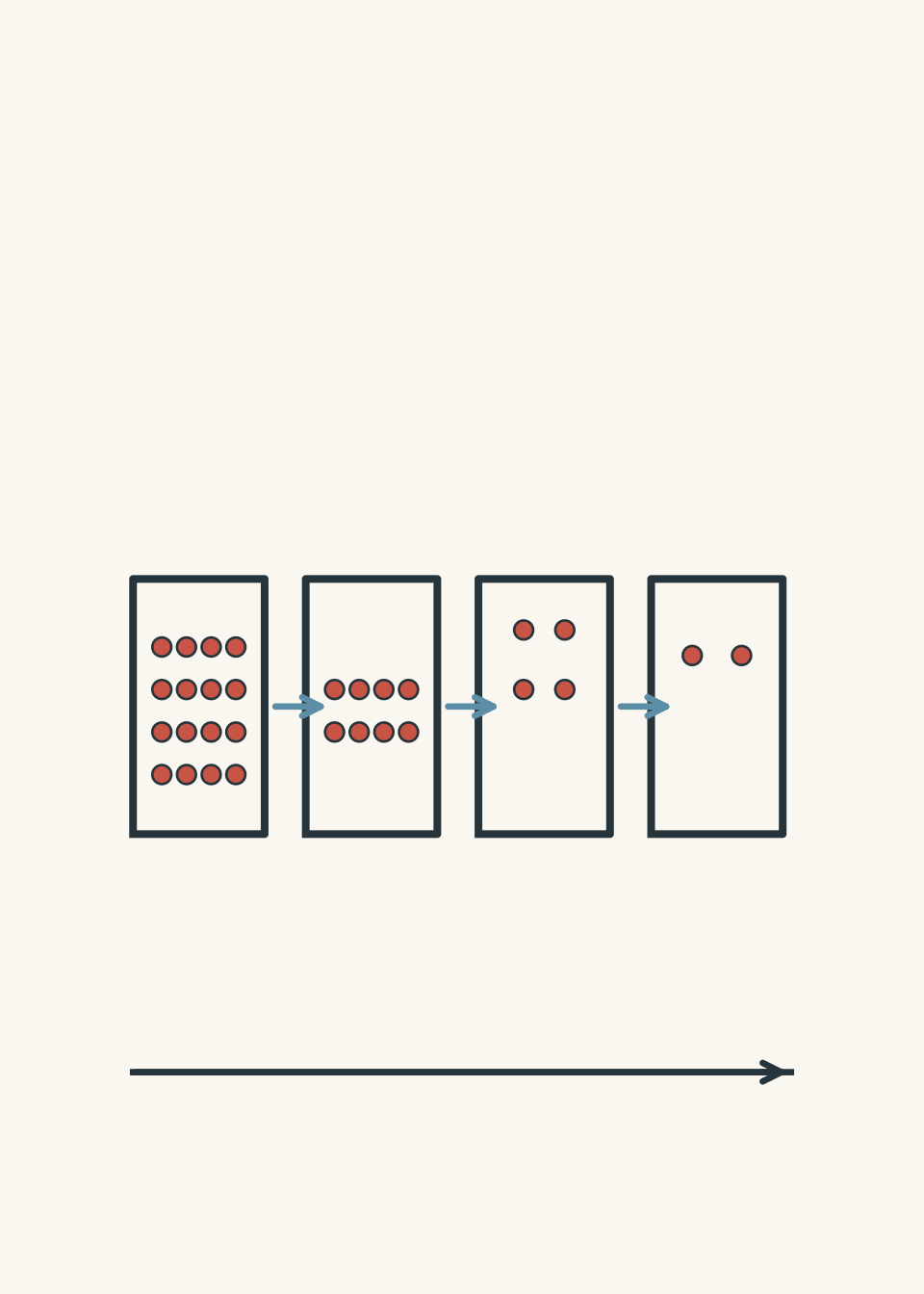
The key idea is that radioactive decay is random for individual nuclei but predictable for large numbers of nuclei. The decay constant connects these two ideas. It tells us how likely each nucleus is to decay in a given amount of time.
01Building the idea of radioactive decay
Think about a large crowd leaving a stadium.
If each person has the same small chance of leaving in the next minute, you cannot predict exactly which person walks out next. However, you can make a very good prediction about the number of people who leave each minute because the crowd is large.
Radioactive nuclei behave in a similar way.
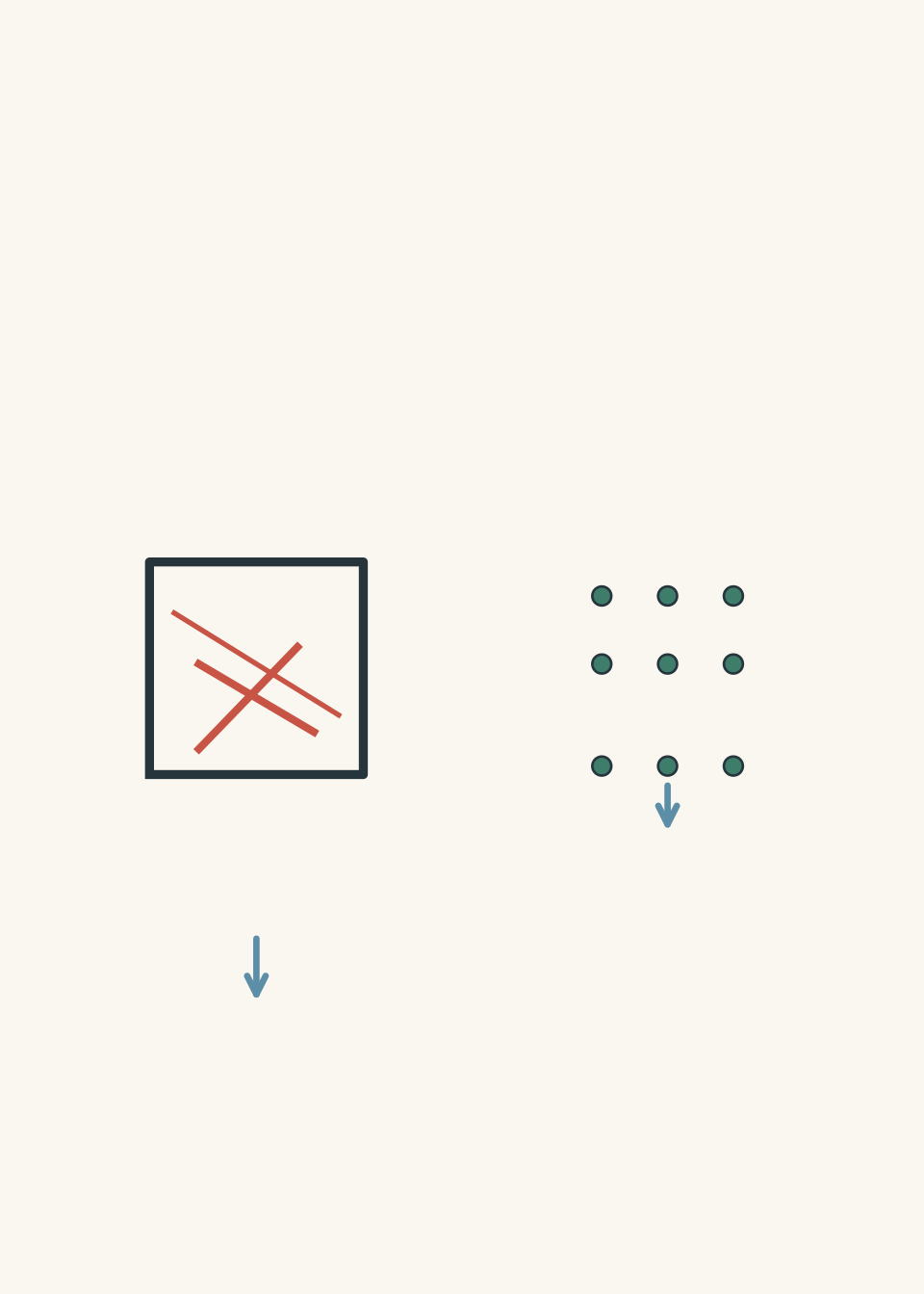
Each unstable nucleus has a probability of decaying. It does not “wait” until a particular age and then decay. A nucleus that has existed for 1 second has the same chance of decaying in the next second as a nucleus that has existed for 1000 years.
This is called a memoryless process.
A common prediction is:
“If half the nuclei decay, the remaining nuclei should become more stable because they have survived longer.”
That feels reasonable because many everyday objects do age. A phone battery gets weaker after years of use. A car part wears down with time.
Radioactive nuclei are different. The remaining nuclei are not “tougher survivors”. They have exactly the same probability of decay as they did before.
02From probability to the decay constant
The decay constant, represented by the symbol \( \lambda \) (lambda), measures the probability of decay per unit time.
A larger \( \lambda \) means:
- individual nuclei are more likely to decay in a given time,
- the sample decreases faster,
- the half-life is shorter.
A smaller \( \lambda \) means:
- individual nuclei are less likely to decay,
- the sample decreases more slowly,
- the half-life is longer.
The relationship between decay constant and half-life is:
\[ \lambda = \frac{\ln 2}{t_{1/2}} \]
where:
- \( \lambda \) is the decay constant in \( \text{s}^{-1} \) (or another unit of inverse time),
- \( \ln 2 \) is the natural logarithm of 2, approximately \(0.693\),
- \( t_{1/2} \) is the half-life in seconds (or the same time unit used for \( \lambda \)).
Why does \(0.693\) appear?
The amount of radioactive material decreases exponentially. After one half-life, the amount remaining is:
\[ \frac{1}{2} \]
The exponential decay model is:
\[ N = N_0 e^{-\lambda t} \]
where:
- \(N\) is the number of undecayed nuclei after time \(t\),
- \(N_0\) is the original number of nuclei,
- \(e\) is Euler’s number, approximately \(2.718\),
- \(t\) is time.
At one half-life:
\[ \frac{N}{N_0}=\frac{1}{2} \]
so:
\[ \frac{1}{2}=e^{-\lambda t_{1/2}} \]
Solving this gives:
\[ \lambda t_{1/2}=\ln 2 \]
and therefore:
\[ \lambda=\frac{\ln 2}{t_{1/2}} \]
The equation is not a new rule about individual atoms. It is a mathematical description of the pattern produced by huge numbers of random events.
03Half-life as a shortcut
Half-life is often easier to picture than the decay constant.
If a sample starts with \(N_0\) nuclei:
- after one half-life: \(N=\frac{N_0}{2}\)
- after two half-lives: \(N=\frac{N_0}{4}\)
- after three half-lives: \(N=\frac{N_0}{8}\)
The number does not decrease by the same amount each time. It decreases by the same fraction.
For example, a sample might change like this:
| Time passed | Fraction remaining |
|---|---|
| 0 half-lives | \(1\) |
| 1 half-life | \(\frac{1}{2}\) |
| 2 half-lives | \(\frac{1}{4}\) |
| 3 half-lives | \(\frac{1}{8}\) |
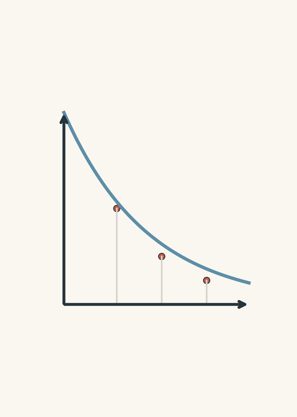
This is where students often make a mistake. They see “half-life” and assume a sample always loses half its original amount each time.
That is false.
After the first half-life, half of the original sample has decayed. After the second half-life, only another quarter of the original sample has decayed.
04Connecting decay constant to activity
Radioactive activity is the rate at which nuclei decay.
It is measured in becquerels (Bq), where:
\[ 1\text{ Bq}=1\text{ decay per second} \]
The activity \(A\) is related to the number of undecayed nuclei:
\[ A=\lambda N \]
where:
- \(A\) is activity in becquerels,
- \( \lambda \) is the decay constant,
- \(N\) is the number of undecayed nuclei.
This equation gives an important physical meaning to \( \lambda \).
If two samples contain the same number of radioactive nuclei, the one with the larger decay constant has the greater activity because each nucleus has a greater chance of decaying.
However, a small sample of a fast-decaying isotope can have lower activity than a huge sample of a slow-decaying isotope. The number of nuclei matters too.
05Worked example: Finding the decay constant from a half-life
A radioactive isotope has a half-life of 8.0 days. Calculate its decay constant in units of \( \text{day}^{-1} \).
Step 1
The formula is:
\[ \lambda=\frac{\ln 2}{t_{1/2}} \]
The half-life is given as:
\[ t_{1/2}=8.0\text{ days} \]
Step 2
\[ \lambda=\frac{0.693}{8.0} \]
Step 3
\[ \lambda=0.0866\text{ day}^{-1} \]
Step 4
The decay constant is \(0.0866\text{ day}^{-1}\). This means that each nucleus has a probability described by this decay constant of decaying per day, and the entire sample follows this average decay pattern.
06Worked example: Using decay constant to find activity
A sample contains \(3.0\times10^{20}\) radioactive nuclei. Its decay constant is \(2.0\times10^{-6}\text{ s}^{-1}\). Calculate its activity.
Step 1
\[ A=\lambda N \]
where:
- \(A\) is activity in Bq,
- \( \lambda=2.0\times10^{-6}\text{ s}^{-1}\),
- \(N=3.0\times10^{20}\).
Step 2
\[ A=(2.0\times10^{-6})(3.0\times10^{20}) \]
Step 3
\[ A=6.0\times10^{14}\text{ Bq} \]
Step 4
The sample undergoes \(6.0\times10^{14}\) decays every second on average. Individual nuclei still decay randomly, but the large number of nuclei creates a predictable activity.
07Where the simple model needs more care
The equations above assume:
- the sample is not being added to or removed from,
- the isotope is decaying naturally,
- the decay constant stays constant,
- there are enough nuclei for statistical patterns to be reliable.
For a single nucleus, saying “the probability of decay is \( \lambda \)” is not quite complete. The probability depends on the time interval being considered. The decay constant is a rate, not a prediction that a particular atom will decay at a particular moment.
This distinction is why radioactive decay is both random and predictable.
You cannot say:
“That nucleus will decay tomorrow.”
You can say:
“Out of a very large number of similar nuclei, we expect a predictable fraction to decay over that time.”
08Connection to nuclear equations
Decay constant and half-life describe how quickly a radioactive sample changes. To understand what it changes into, you need to look at the type of radiation and the nuclear reaction itself.
For example, alpha decay changes the nucleus by releasing an alpha particle. The conservation rules behind these reactions are explained further in Alpha decay: nuclear equations and radiation properties.
09Questions and solutions
Question 1
A radioactive isotope has a half-life of 12 hours. Calculate its decay constant in units of \( \text{hour}^{-1} \).
Solution 1
The decay constant is \(0.0578\text{ hour}^{-1}\). It is found by converting the half-life into a decay rate using:
\[ \lambda=\frac{\ln 2}{t_{1/2}} \]
Substitute:
\[ \lambda=\frac{0.693}{12} \]
\[ \lambda=0.0578\text{ hour}^{-1} \]
The result means that the isotope has a greater decay probability per hour than an isotope with a smaller decay constant, but it does not mean every nucleus decays at that rate.
Question 2
A sample initially contains \(8.0\times10^{18}\) radioactive nuclei. Its half-life is 5.0 days. How many nuclei remain after 15 days?
Solution 2
The sample has \(1.0\times10^{18}\) nuclei remaining after 15 days. The key step is recognising that 15 days represents three half-lives.
First calculate the number of half-lives:
\[ \text{number of half-lives}=\frac{15}{5.0}=3 \]
Apply the halving pattern:
\[ N=N_0\left(\frac{1}{2}\right)^3 \]
\[ N=(8.0\times10^{18})\left(\frac{1}{8}\right) \]
\[ N=1.0\times10^{18} \]
The tempting mistake is to subtract half the original amount three times. Radioactive decay halves the remaining amount, not the original amount.
Question 3
Two radioactive samples contain the same number of nuclei. Sample A has a half-life of 2 days, and Sample B has a half-life of 20 days. Explain which sample has the greater initial activity and why.
Solution 3
Sample A has the greater initial activity because it has the larger decay constant. Activity depends on:
\[ A=\lambda N \]
Both samples have the same \(N\), so the comparison depends only on \( \lambda \).
Using:
\[ \lambda=\frac{\ln2}{t_{1/2}} \]
a shorter half-life gives a larger decay constant. Since Sample A has the shorter half-life, more nuclei decay each second initially.
The trap is thinking that the sample with the longer lifetime has more “radioactivity stored”. Radioactive activity is about decay rate, not how long the isotope survives.
Question 4
A scientist measures the activity of a radioactive sample and finds it has decreased from \(1600\text{ Bq}\) to \(200\text{ Bq}\) over 18 hours. The sample has not lost any material. Determine the half-life and explain why the result does not mean every nucleus waited 6 hours before decaying.
Solution 4
The half-life is 6.0 hours because the activity has reduced by three successive halvings.
The activity changes as:
\[ 1600\text{ Bq}\rightarrow800\text{ Bq}\rightarrow400\text{ Bq}\rightarrow200\text{ Bq} \]
This is three half-lives.
\[ 3t_{1/2}=18\text{ h} \]
\[ t_{1/2}=6.0\text{ h} \]
The second part is important: individual nuclei did not follow a schedule. Some decayed earlier, and some remained undecayed after 18 hours. The half-life describes the statistical behaviour of the whole sample.
Question 5
A student argues:
“Isotope X has a shorter half-life than isotope Y, so after a very long time isotope X must have fewer undecayed nuclei than isotope Y.”
Both samples start with the same number of nuclei. Evaluate this statement.
Solution 5
The statement is not always correct because the time being considered determines the result.
A shorter half-life means isotope X has a larger decay constant and decreases faster. This means that for many times after the start, X will have fewer undecayed nuclei.
However, after an extremely long time, both samples approach zero remaining nuclei. The statement uses the word “must”, which is too strong.
The exact relationship is:
\[ N=N_0e^{-\lambda t} \]
Because isotope X has a larger \( \lambda \), its curve falls faster. But both values depend on the chosen time \(t\). At \(t=0\), they are equal. At very large \(t\), both are extremely close to zero.
The deeper idea is that a larger decay constant changes the speed of the process, not the final destination. Radioactive decay is not a race where one sample eventually reaches a different endpoint; it is a continuous probability process governed by the decay constant. This same idea helps when comparing different radioactive tracers in nuclear physics applications.