
Determining Keq for the Iron(III) Thiocyanate Equilibrium
Learn how absorbance data, calibration curves, dilution calculations, and equilibrium concentrations are used to determine Keq for the iron(III) thiocyanate system.
You mix iron(III) ions with thiocyanate ions and the solution turns red. Make a second mixture with different starting concentrations and it becomes a deeper red.
Predict this before going further: does the darker mixture have a larger equilibrium constant?
No. If both mixtures are at the same temperature and under the same solution conditions, they have the same \(K_\text{eq}\). The darker mixture simply contains a different equilibrium concentration of the red complex. The experimental problem is therefore not “which tube is redder?” It is: how can we turn that colour into an equilibrium concentration, then use it to work out all three concentrations needed for \(K_\text{eq}\)?
That is what the iron(III) thiocyanate experiment does.
01The equilibrium we are trying to measure
The simplified equilibrium is
\[ \ce{Fe^3+(aq) + SCN^-(aq) <=> FeSCN^2+(aq)} \]
The product, \(\mathrm{FeSCN}^{2+}\), is a strongly coloured red complex ion. Potassium ions from \(\ce{KSCN}\) and nitrate ions from \(\ce{Fe(NO3)3}\) are spectators, so they do not appear in the equilibrium equation.
For this 1:1:1 reaction,
\[ K_\text{eq} = \frac{[\mathrm{FeSCN}^{2+}]_\text{eq}} {[\mathrm{Fe}^{3+}]_\text{eq}[\mathrm{SCN}^{-}]_\text{eq}} \]
Square brackets mean concentration in \(\mathrm{mol\,L^{-1}}\), and the subscript “eq” reminds us that these must be equilibrium concentrations, not the concentrations in the stock bottles and not even the concentrations immediately after mixing.
That distinction is where a lot of mistakes begin.
Suppose you initially mix \(1.00\times10^{-3}\ \mathrm{mol\,L^{-1}}\) of \(\mathrm{Fe}^{3+}\) with \(2.00\times10^{-4}\ \mathrm{mol\,L^{-1}}\) of \(\mathrm{SCN}^{-}\). It would be tempting to put those two numbers straight into the denominator of \(K_\text{eq}\).
But some of each reactant has already formed \(\mathrm{FeSCN}^{2+}\). We need to find how much product formed, then subtract that amount from each reactant.
The current NSW Chemistry Stage 6 equilibrium content includes both the iron(III) nitrate-potassium thiocyanate system as a reversible reaction and quantitative determination of equilibrium constants.
02The first measurement idea: just look at the colour
A simple experiment could use several identical test tubes.
You prepare mixtures containing different known amounts of \(\mathrm{FeSCN}^{2+}\), place them side by side, and compare their redness with the unknown equilibrium mixture.
What should happen as \([\mathrm{FeSCN}^{2+}]\) increases?
The solution should absorb more light and appear more intensely coloured. That prediction works well enough to show that concentration and colour intensity are connected.
But your eye is a pretty ordinary measuring instrument.
Two very similar reds are difficult to distinguish. Ambient light changes your judgement. More importantly, the apparent darkness also depends on how far light travels through the solution.
Think about cordial. The same cordial can look darker through the long side of a rectangular container than through the short side. The concentration has not changed; the light simply travelled through more liquid.
That analogy is useful because the same thing happens in spectroscopy: both concentration and light-path length affect absorbance. It breaks down once we need precise numbers, because your eyes do not give a reliable numerical measure of absorbed light.
So the design needs an upgrade.
03The revised design: make the light do the measuring
A spectrophotometer replaces “that one looks a bit redder” with a measured absorbance.
Spatially, the experiment looks like this:
- A light source produces light.
- A wavelength selector chooses a narrow range of wavelengths.
- That light passes through the solution inside a cuvette.
- A detector measures how much light emerges from the other side.
- The instrument converts the loss of light into an absorbance, \(A\).
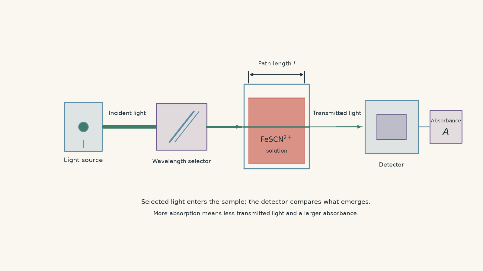
Iron(III) thiocyanate experiments commonly measure near \(447\)-\(450\ \mathrm{nm}\), where the red complex strongly absorbs blue light.
Under suitable conditions, the Beer-Lambert law gives
\[ A=\varepsilon lc \]
where:
- \(A\) is absorbance, which has no unit,
- \(\varepsilon\) is the molar absorptivity at the chosen wavelength,
- \(l\) is the light path through the sample, usually the width of the cuvette in \(\mathrm{cm}\), and
- \(c\) is the concentration of the absorbing species in \(\mathrm{mol\,L^{-1}}\).
If the same cuvette type and wavelength are used every time, \(\varepsilon\) and \(l\) stay constant. Absorbance then becomes directly proportional to concentration.
Double the concentration, and, within the useful linear range, you expect roughly double the absorbance.
04The calibration problem: how do you make a “known” equilibrium product?
There is an awkward circular problem.
We want to use absorbance to determine \([\mathrm{FeSCN}^{2+}]\). To calibrate the spectrophotometer, however, we first need solutions with known \([\mathrm{FeSCN}^{2+}]\).
But the reaction is reversible. If you simply mix similar amounts of \(\mathrm{Fe}^{3+}\) and \(\mathrm{SCN}^{-}\), you do not know in advance how much becomes product.
The trick is to prepare the calibration standards differently from the actual equilibrium mixtures.
Use a very large excess of \(\mathrm{Fe}^{3+}\) and a small, known amount of \(\mathrm{SCN}^{-}\). The large iron(III) concentration drives the equilibrium strongly towards products, so at the school-experiment level we approximate almost all of the limiting \(\mathrm{SCN}^{-}\) as becoming \(\mathrm{FeSCN}^{2+}\). This excess-reactant method is commonly used to prepare calibration standards for the experiment.
So, approximately,
\[ [\mathrm{FeSCN}^{2+}]_\text{standard} \approx [\mathrm{SCN}^{-}]_\text{initial, diluted} \]
Notice the word approximately. We have deliberately created conditions where an approximation that would be wrong in the equilibrium samples becomes useful in the calibration standards.
A quick calibration-scale calculation
Suppose \(1.00\ \mathrm{mL}\) of \(2.00\times10^{-3}\ \mathrm{mol\,L^{-1}}\) \(\ce{KSCN}\) is diluted to \(25.00\ \mathrm{mL}\) in a large excess of \(\mathrm{Fe}^{3+}\).
The number of moles of \(\mathrm{SCN}^{-}\) added is
\[ n=cV =(2.00\times10^{-3})(1.00\times10^{-3}) =2.00\times10^{-6}\ \mathrm{mol} \]
If essentially all of it forms the red complex,
\[ [\mathrm{FeSCN}^{2+}] \approx \frac{2.00\times10^{-6}}{0.02500} = 8.00\times10^{-5}\ \mathrm{mol\,L^{-1}} \]
That gives one known calibration point.
Prepare several standards, measure their absorbances, and plot absorbance against concentration.
The experimental calibration might have the form
\[ A=mc+b \]
where \(m\) is the gradient and \(b\) is the intercept. If the blank correction is perfect and Beer-Lambert behaviour is ideal, \(b\) should be close to zero. In real experimental data, use the actual fitted line rather than casually pretending the intercept does not exist.
05What the blank is doing
Before measuring the red complex, the spectrophotometer needs a reference.
A blank measures absorption caused by things other than the species we actually want: the solvent, cuvette, and ideally any background from the chemical medium.
This matters because \(\mathrm{Fe}^{3+}\) solutions themselves can have some colour. A suitable blank prevents background absorption from being mistaken for extra \(\mathrm{FeSCN}^{2+}\).
The cuvette also needs to be clean. A fingerprint is not chemically interesting, but the detector does not know that. If it blocks extra light, the instrument can report an absorbance that is too high.
06Preparing the real equilibrium mixture
The calibration standards deliberately use a huge excess of iron(III). The equilibrium mixtures do not.
Here we mix measured amounts of \(\mathrm{Fe}^{3+}\) and \(\mathrm{SCN}^{-}\), allow the reversible reaction to establish equilibrium, and measure the red complex without assuming the reaction went to completion.
There are two concentration calculations to keep separate.
First, calculate the concentrations immediately after dilution and mixing. If a stock solution with concentration \(c_\text{stock}\) contributes volume \(V_\text{stock}\) to a final volume \(V_\text{total}\),
\[ c_\text{initial} = c_\text{stock} \frac{V_\text{stock}}{V_\text{total}} \]
These are the initial concentrations for the ICE table.
Second, use the measured absorbance and calibration curve to find the equilibrium concentration of \(\mathrm{FeSCN}^{2+}\).
If no red complex was deliberately present before mixing and the measured equilibrium product concentration is \(x\), the stoichiometry gives
| Species | Initial concentration | Change | Equilibrium concentration |
|---|---|---|---|
| \(\mathrm{Fe}^{3+}\) | \(F_0\) | \(-x\) | \(F_0-x\) |
| \(\mathrm{SCN}^{-}\) | \(S_0\) | \(-x\) | \(S_0-x\) |
| \(\mathrm{FeSCN}^{2+}\) | \(0\) | \(+x\) | \(x\) |
The reason the same \(x\) appears three times is the 1:1:1 stoichiometric ratio.
Once those equilibrium concentrations are known,
\[ K_\text{eq} = \frac{x}{(F_0-x)(S_0-x)} \]
That is the whole calculation. The difficult part is keeping straight what was measured, what was calculated from dilution, and what was inferred using stoichiometry.
07Worked example: Determine \(K_\text{eq}\) from absorbance
An equilibrium mixture initially contains \(1.00\times10^{-3}\ \mathrm{mol\,L^{-1}}\) \(\mathrm{Fe}^{3+}\) and \(2.00\times10^{-4}\ \mathrm{mol\,L^{-1}}\) \(\mathrm{SCN}^{-}\). Its measured absorbance is \(0.287\). The calibration equation is \(A=(4.70\times10^3)c+0.005\), where \(c\) is \([\mathrm{FeSCN}^{2+}]\) in \(\mathrm{mol\,L^{-1}}\). Determine \(K_\text{eq}\).
Step 1
\[ \begin{aligned} 0.287&=(4.70\times10^3)c+0.005\\ c&=\frac{0.287-0.005}{4.70\times10^3}\\ &=6.00\times10^{-5}\ \mathrm{mol\,L^{-1}} \end{aligned} \]
So,
\[ [\mathrm{FeSCN}^{2+}]_\text{eq} = 6.00\times10^{-5}\ \mathrm{mol\,L^{-1}} \]
Step 2
Formation of \(6.00\times10^{-5}\ \mathrm{mol\,L^{-1}}\) of product consumes the same concentration of each reactant.
\[ \begin{aligned} [\mathrm{Fe}^{3+}]_\text{eq} &= 1.00\times10^{-3}-6.00\times10^{-5}\\ &= 9.40\times10^{-4}\ \mathrm{mol\,L^{-1}} \end{aligned} \]
and
\[ \begin{aligned} [\mathrm{SCN}^{-}]_\text{eq} &= 2.00\times10^{-4}-6.00\times10^{-5}\\ &= 1.40\times10^{-4}\ \mathrm{mol\,L^{-1}} \end{aligned} \]
Step 3
\[ \begin{aligned} K_\text{eq} &= \frac{6.00\times10^{-5}} {(9.40\times10^{-4})(1.40\times10^{-4})}\\ &=4.56\times10^2 \end{aligned} \]
Step 4
The measured value is
\[ K_\text{eq}\approx456 \]
The equilibrium is substantially product-favoured, but the reaction has clearly not gone to completion. Both reactants remain in measurable concentrations.
The tempting mistake here is to put the two initial concentrations directly into the denominator. Doing that ignores the material already consumed to form the red complex.
08Worked example: Include the mixing dilution first
A student mixes \(5.00\ \mathrm{mL}\) of \(2.00\times10^{-3}\ \mathrm{mol\,L^{-1}}\) \(\mathrm{Fe}^{3+}\) with \(3.00\ \mathrm{mL}\) of \(2.00\times10^{-3}\ \mathrm{mol\,L^{-1}}\) \(\mathrm{SCN}^{-}\), then dilutes the mixture to \(10.00\ \mathrm{mL}\). At equilibrium, its absorbance is \(0.816\). The calibration equation is \(A=(4.20\times10^3)c+0.006\). Calculate \(K_\text{eq}\).
Step 1
For \(\mathrm{Fe}^{3+}\),
\[ \begin{aligned} [\mathrm{Fe}^{3+}]_0 &= (2.00\times10^{-3}) \frac{5.00}{10.00}\\ &= 1.00\times10^{-3}\ \mathrm{mol\,L^{-1}} \end{aligned} \]
For \(\mathrm{SCN}^{-}\),
\[ \begin{aligned} [\mathrm{SCN}^{-}]_0 &= (2.00\times10^{-3}) \frac{3.00}{10.00}\\ &= 6.00\times10^{-4}\ \mathrm{mol\,L^{-1}} \end{aligned} \]
The stock concentrations are not the ICE-table concentrations because both stock solutions have been diluted.
Step 2
\[ \begin{aligned} 0.816&=(4.20\times10^3)c+0.006\\ c&=\frac{0.816-0.006}{4.20\times10^3}\\ &=1.93\times10^{-4}\ \mathrm{mol\,L^{-1}} \end{aligned} \]
Therefore,
\[ [\mathrm{FeSCN}^{2+}]_\text{eq} = 1.93\times10^{-4}\ \mathrm{mol\,L^{-1}} \]
Step 3
\[ [\mathrm{Fe}^{3+}]_\text{eq} = 1.00\times10^{-3}-1.93\times10^{-4} = 8.07\times10^{-4}\ \mathrm{mol\,L^{-1}} \]
\[ [\mathrm{SCN}^{-}]_\text{eq} = 6.00\times10^{-4}-1.93\times10^{-4} = 4.07\times10^{-4}\ \mathrm{mol\,L^{-1}} \]
Step 4
\[ \begin{aligned} K_\text{eq} &= \frac{1.93\times10^{-4}} {(8.07\times10^{-4})(4.07\times10^{-4})}\\ &\approx5.87\times10^2 \end{aligned} \]
So the experimental result is
\[ K_\text{eq}\approx587 \]
Step 5
One measurement does not establish a perfect value. You would normally calculate \(K_\text{eq}\) for several mixtures with different starting concentrations. Similar values provide evidence that the equilibrium model and measurements are behaving reasonably.
Blindly averaging wildly different values is not a fix. Large disagreement is evidence that something in the method, calibration, temperature control, or chemical model needs checking.
09What the experiment actually demonstrates
There are several layers of reasoning in this experiment.
The direct observation is the absorbance.
Beer-Lambert behaviour lets us interpret that absorbance as a concentration of the coloured species.
Reaction stoichiometry then lets us infer the concentrations of the two reactants that remain.
Only after all three equilibrium concentrations are known do we calculate \(K_\text{eq}\).
This separation matters. A spectrophotometer does not directly measure the equilibrium constant. It does not even directly measure moles. It measures light.
The chemistry connects that light measurement to \(K_\text{eq}\).
10Why the chemical conditions need to stay controlled
Temperature must stay reasonably constant because changing temperature can change the equilibrium constant itself.
This is different from changing a reactant concentration at constant temperature. Changing concentration disturbs the equilibrium position, but after the system readjusts, the same \(K_\text{eq}\) applies.
Iron(III) chemistry also gives us another reason to control the solution medium. \(\mathrm{Fe}^{3+}\) can undergo hydrolysis in water, so many experimental procedures use an acidic medium to suppress competing iron hydrolysis reactions.
If some of the iron you count as “free \(\mathrm{Fe}^{3+}\)” is actually tied up in another species, the simple ICE table no longer describes the whole chemical system.
Where the simple model stops being exact
For HSC calculations, we normally model the coloured equilibrium as
\[ \ce{Fe^3+ + SCN^- <=> FeSCN^2+} \]
That is a useful controlled model, not a claim that every iron and thiocyanate ion in every possible solution participates only in that one equilibrium.
At higher thiocyanate concentrations, additional iron-thiocyanate complexes can form. More advanced experiments therefore use dilute, controlled solutions so that the 1:1 complex is the dominant species and the simple treatment remains useful.
There is a second layer of precision too. At HSC level we calculate \(K_\text{eq}\) using concentrations. In more advanced physical chemistry, equilibrium constants are formally defined using activities, which account for non-ideal behaviour in ionic solutions.
You do not need activity calculations for the HSC. You do need to understand why changing the chemical medium carelessly can make experimentally determined values less consistent.
11Common experimental errors and what they do
| Problem | What happens to the calculation? | Why |
|---|---|---|
| Using stock concentrations instead of diluted initial concentrations | \(K_\text{eq}\) is usually underestimated | The denominator uses reactant concentrations that are too large |
| Fingerprints or droplets on the cuvette increase measured absorbance | \(K_\text{eq}\) is usually overestimated | Calculated \([\mathrm{FeSCN}^{2+}]\) is too large, while the calculated remaining reactants become too small |
| Forgetting a positive calibration intercept | Product concentration is overestimated | Some absorbance that belongs to the intercept is incorrectly assigned to \(\mathrm{FeSCN}^{2+}\) |
| Calibration standards do not convert nearly all \(\mathrm{SCN}^{-}\), but you assume they do | Usually overestimates product concentrations in unknowns | The standards are labelled with concentrations larger than their true \([\mathrm{FeSCN}^{2+}]\), making the fitted calibration gradient too small |
| Different temperatures are used for different trials | The trials may genuinely have different \(K_\text{eq}\) values | Temperature can change the equilibrium constant |
| Background absorbance is not blanked properly | Creates a systematic error in \([\mathrm{FeSCN}^{2+}]\) | The detector cannot tell background absorption from absorption by the complex |
| Using initial reactant concentrations directly in the \(K_\text{eq}\) expression | \(K_\text{eq}\) is underestimated | Reactant concentrations at equilibrium are lower than their initial values |
A useful exam habit is to trace an error through the entire calculation rather than saying something vague like “the result becomes inaccurate”.
For example:
higher measured \(A\)
\[ \longrightarrow \text{higher calculated }[\mathrm{FeSCN}^{2+}] \]
\[ \longrightarrow \text{lower calculated }[\mathrm{Fe}^{3+}]\text{ and }[\mathrm{SCN}^{-}] \]
\[ \longrightarrow \text{larger numerator and smaller denominator} \]
\[ \longrightarrow \text{calculated }K_\text{eq}\text{ too high} \]
That chain is much stronger than simply writing “human error”.
12Questions and solutions
Question 1
At equilibrium, a solution has
\[ [\mathrm{Fe}^{3+}]=8.00\times10^{-4}\ \mathrm{mol\,L^{-1}} \]
\[ [\mathrm{SCN}^{-}]=2.00\times10^{-4}\ \mathrm{mol\,L^{-1}} \]
and
\[ [\mathrm{FeSCN}^{2+}]=1.20\times10^{-4}\ \mathrm{mol\,L^{-1}} \]
Calculate \(K_\text{eq}\) and interpret its magnitude.
Solution 1
The equilibrium constant is \(7.50\times10^2\), indicating a product-favoured equilibrium under these conditions, although reactants are still present.
The equilibrium expression is
\[ K_\text{eq} = \frac{[\mathrm{FeSCN}^{2+}]} {[\mathrm{Fe}^{3+}][\mathrm{SCN}^{-}]} \]
Substitute the equilibrium concentrations:
\[ \begin{aligned} K_\text{eq} &= \frac{1.20\times10^{-4}} {(8.00\times10^{-4})(2.00\times10^{-4})}\\ &= \frac{1.20\times10^{-4}} {1.60\times10^{-7}}\\ &= 7.50\times10^2 \end{aligned} \]
A common trap is to interpret a large \(K_\text{eq}\) as meaning “all reactants are gone”. It does not. The measured equilibrium concentrations explicitly show that both reactants remain.
Question 2
A student mixes \(5.00\ \mathrm{mL}\) of \(2.00\times10^{-3}\ \mathrm{mol\,L^{-1}}\) \(\mathrm{Fe}^{3+}\) with \(2.00\ \mathrm{mL}\) of \(2.00\times10^{-3}\ \mathrm{mol\,L^{-1}}\) \(\mathrm{SCN}^{-}\), then dilutes the mixture to \(10.00\ \mathrm{mL}\).
The equilibrium absorbance is \(0.730\), and the calibration equation is
\[ A=(4.80\times10^3)c+0.010 \]
where \(c=[\mathrm{FeSCN}^{2+}]\) in \(\mathrm{mol\,L^{-1}}\).
Calculate \(K_\text{eq}\).
Solution 2
The equilibrium constant is approximately \(7.06\times10^2\).
First calculate the initial concentrations after dilution.
For iron(III),
\[ [\mathrm{Fe}^{3+}]_0 = (2.00\times10^{-3}) \frac{5.00}{10.00} = 1.00\times10^{-3}\ \mathrm{mol\,L^{-1}} \]
For thiocyanate,
\[ [\mathrm{SCN}^{-}]_0 = (2.00\times10^{-3}) \frac{2.00}{10.00} = 4.00\times10^{-4}\ \mathrm{mol\,L^{-1}} \]
Now use the calibration equation:
\[ \begin{aligned} 0.730&=(4.80\times10^3)c+0.010\\ c&=\frac{0.730-0.010}{4.80\times10^3}\\ &=1.50\times10^{-4}\ \mathrm{mol\,L^{-1}} \end{aligned} \]
Therefore,
\[ [\mathrm{FeSCN}^{2+}]_\text{eq} = 1.50\times10^{-4}\ \mathrm{mol\,L^{-1}} \]
The remaining reactant concentrations are
\[ [\mathrm{Fe}^{3+}]_\text{eq} = 1.00\times10^{-3}-1.50\times10^{-4} = 8.50\times10^{-4}\ \mathrm{mol\,L^{-1}} \]
and
\[ [\mathrm{SCN}^{-}]_\text{eq} = 4.00\times10^{-4}-1.50\times10^{-4} = 2.50\times10^{-4}\ \mathrm{mol\,L^{-1}} \]
Hence,
\[ \begin{aligned} K_\text{eq} &= \frac{1.50\times10^{-4}} {(8.50\times10^{-4})(2.50\times10^{-4})}\\ &= 7.06\times10^2 \end{aligned} \]
There are two tempting shortcuts here. One is forgetting that the stock solutions were diluted. The other is ignoring the \(0.010\) intercept. Either changes the final equilibrium concentrations before the \(K_\text{eq}\) calculation has even begun.
Question 3
At the measurement wavelength, a reagent blank has an absorbance of \(0.040\). A student accidentally measures an equilibrium sample relative to water instead of the reagent blank and obtains \(A=0.560\).
The correctly blanked calibration relationship is
\[ A=(5.00\times10^3)c \]
The equilibrium mixture initially contained
\[ [\mathrm{Fe}^{3+}]_0=1.00\times10^{-3}\ \mathrm{mol\,L^{-1}} \]
and
\[ [\mathrm{SCN}^{-}]_0=3.00\times10^{-4}\ \mathrm{mol\,L^{-1}} \]
Calculate the correct \(K_\text{eq}\), calculate the value obtained if the blank is ignored, and explain the direction of the error.
Solution 3
The correctly calculated equilibrium constant is approximately \(5.92\times10^2\); ignoring the blank gives approximately \(6.71\times10^2\), so the error causes \(K_\text{eq}\) to be overestimated.
The absorbance caused by the complex alone is
\[ A_\text{complex} = 0.560-0.040 = 0.520 \]
Therefore,
\[ [\mathrm{FeSCN}^{2+}]_\text{eq} = \frac{0.520}{5.00\times10^3} = 1.04\times10^{-4}\ \mathrm{mol\,L^{-1}} \]
The correct equilibrium reactant concentrations are
\[ [\mathrm{Fe}^{3+}]_\text{eq} = 1.00\times10^{-3}-1.04\times10^{-4} = 8.96\times10^{-4}\ \mathrm{mol\,L^{-1}} \]
and
\[ [\mathrm{SCN}^{-}]_\text{eq} = 3.00\times10^{-4}-1.04\times10^{-4} = 1.96\times10^{-4}\ \mathrm{mol\,L^{-1}} \]
So,
\[ \begin{aligned} K_\text{eq} &= \frac{1.04\times10^{-4}} {(8.96\times10^{-4})(1.96\times10^{-4})}\\ &\approx5.92\times10^2 \end{aligned} \]
If the student ignores the background and treats the full \(0.560\) as absorption by the complex,
\[ [\mathrm{FeSCN}^{2+}]_\text{wrong} = \frac{0.560}{5.00\times10^3} = 1.12\times10^{-4}\ \mathrm{mol\,L^{-1}} \]
This gives
\[ [\mathrm{Fe}^{3+}]_\text{wrong} = 8.88\times10^{-4}\ \mathrm{mol\,L^{-1}} \]
and
\[ [\mathrm{SCN}^{-}]_\text{wrong} = 1.88\times10^{-4}\ \mathrm{mol\,L^{-1}} \]
Therefore,
\[ K_{\text{eq, wrong}} = \frac{1.12\times10^{-4}} {(8.88\times10^{-4})(1.88\times10^{-4})} \approx6.71\times10^2 \]
The important reasoning is not merely “absorbance was too high”. The falsely high absorbance makes the calculated product concentration too high. Because product formation is then subtracted from both reactants, both denominator concentrations also become too low.
The numerator increases while the denominator decreases. Both effects push the calculated \(K_\text{eq}\) upwards.
Question 4
A calibration is prepared by assuming that every mole of \(\mathrm{SCN}^{-}\) in each standard becomes \(\mathrm{FeSCN}^{2+}\). In reality, the iron(III) excess was not large enough, and only \(80.0\%\) of the assigned \(\mathrm{SCN}^{-}\) concentration became the red complex in every standard.
Assume Beer-Lambert behaviour is otherwise perfect and the student forces the calibration through the origin.
An equilibrium sample has true initial concentrations
\[ [\mathrm{Fe}^{3+}]_0=1.00\times10^{-3}\ \mathrm{mol\,L^{-1}} \]
and
\[ [\mathrm{SCN}^{-}]_0=4.00\times10^{-4}\ \mathrm{mol\,L^{-1}} \]
Its true equilibrium concentration of \(\mathrm{FeSCN}^{2+}\) is \(1.00\times10^{-4}\ \mathrm{mol\,L^{-1}}\).
Determine the product concentration the student would calculate, compare the student’s \(K_\text{eq}\) with the true value, and explain whether a set of very repeatable trials would necessarily reveal this problem.
Solution 4
The student would calculate \([\mathrm{FeSCN}^{2+}]=1.25\times10^{-4}\ \mathrm{mol\,L^{-1}}\), giving \(K_\text{eq}\approx519\) instead of the true value of approximately \(370\). Repeatable trials would not necessarily expose the problem because this is a shared systematic calibration error.
Let the true Beer-Lambert gradient be \(\varepsilon l\).
For a calibration standard labelled with assigned concentration \(c_\text{assigned}\), its actual complex concentration is only
\[ c_\text{true}=0.800c_\text{assigned} \]
Its absorbance is therefore
\[ A=(\varepsilon l)(0.800c_\text{assigned}) \]
When the student plots \(A\) against the incorrectly assigned concentration, the measured gradient becomes
\[ m_\text{student}=0.800\varepsilon l \]
Now consider the unknown sample. Its true product concentration is
\[ 1.00\times10^{-4}\ \mathrm{mol\,L^{-1}} \]
so its absorbance is
\[ A=(\varepsilon l)(1.00\times10^{-4}) \]
The student divides this by the incorrect calibration gradient:
\[ \begin{aligned} c_\text{calculated} &= \frac{(\varepsilon l)(1.00\times10^{-4})} {0.800\varepsilon l}\\ &= 1.25\times10^{-4}\ \mathrm{mol\,L^{-1}} \end{aligned} \]
The true equilibrium constant is
\[ \begin{aligned} K_\text{true} &= \frac{1.00\times10^{-4}} {(1.00\times10^{-3}-1.00\times10^{-4}) (4.00\times10^{-4}-1.00\times10^{-4})}\\ &= \frac{1.00\times10^{-4}} {(9.00\times10^{-4})(3.00\times10^{-4})}\\ &\approx370 \end{aligned} \]
Using the student’s falsely high product concentration gives
\[ \begin{aligned} K_\text{student} &= \frac{1.25\times10^{-4}} {(1.00\times10^{-3}-1.25\times10^{-4}) (4.00\times10^{-4}-1.25\times10^{-4})}\\ &= \frac{1.25\times10^{-4}} {(8.75\times10^{-4})(2.75\times10^{-4})}\\ &\approx519 \end{aligned} \]
The tempting argument is that “if five trials give nearly the same \(K_\text{eq}\), the value must be accurate”.
Not necessarily.
Repeatability mainly tests precision. Every unknown is being interpreted through the same faulty calibration. A systematic error can therefore produce beautifully consistent values that are all wrong.
This is why independent checks on the standards and method matter.
Question 5
At a fixed temperature, an equilibrium mixture has
\[ [\mathrm{Fe}^{3+}]=1.00\times10^{-3}\ \mathrm{mol\,L^{-1}} \]
\[ [\mathrm{SCN}^{-}]=2.00\times10^{-4}\ \mathrm{mol\,L^{-1}} \]
and
\[ [\mathrm{FeSCN}^{2+}]=1.00\times10^{-4}\ \mathrm{mol\,L^{-1}} \]
The calibration is \(A=(5.00\times10^3)c\), so the initial equilibrium absorbance is \(0.500\).
An equal volume of water is suddenly added.
One student says, “Every concentration halves, so the absorbance becomes \(0.250\) and the system is still at equilibrium.”
Another says, “Dilution lowers all the concentrations, so the reaction must shift right to replace the product.”
Determine the reaction quotient immediately after dilution, predict the direction of the subsequent shift, calculate the final equilibrium concentration of \(\mathrm{FeSCN}^{2+}\), and determine the final absorbance. Explain exactly what is wrong with each student’s argument.
Solution 5
Immediately after dilution, \(Q=1000\), which is greater than \(K_\text{eq}=500\), so the system shifts left. After re-establishing equilibrium, \([\mathrm{FeSCN}^{2+}]\approx3.09\times10^{-5}\ \mathrm{mol\,L^{-1}}\) and the absorbance is approximately \(0.155\).
First calculate \(K_\text{eq}\) from the original equilibrium state:
\[ \begin{aligned} K_\text{eq} &= \frac{1.00\times10^{-4}} {(1.00\times10^{-3})(2.00\times10^{-4})}\\ &=500 \end{aligned} \]
Adding an equal volume of water instantly halves every concentration before the reaction has time to respond.
So immediately after dilution,
\[ [\mathrm{Fe}^{3+}]=5.00\times10^{-4}\ \mathrm{mol\,L^{-1}} \]
\[ [\mathrm{SCN}^{-}]=1.00\times10^{-4}\ \mathrm{mol\,L^{-1}} \]
and
\[ [\mathrm{FeSCN}^{2+}]=5.00\times10^{-5}\ \mathrm{mol\,L^{-1}} \]
These are not equilibrium concentrations yet. They describe the disturbed system.
Calculate the reaction quotient:
\[ \begin{aligned} Q &= \frac{5.00\times10^{-5}} {(5.00\times10^{-4})(1.00\times10^{-4})}\\ &=1000 \end{aligned} \]
Since
\[ Q>K_\text{eq} \]
there is too much product relative to reactants for equilibrium at this temperature. The net reaction therefore proceeds to the left.
Let \(y\) be the concentration of \(\mathrm{FeSCN}^{2+}\) that dissociates.
The new equilibrium concentrations are
\[ [\mathrm{FeSCN}^{2+}] = 5.00\times10^{-5}-y \]
\[ [\mathrm{Fe}^{3+}] = 5.00\times10^{-4}+y \]
and
\[ [\mathrm{SCN}^{-}] = 1.00\times10^{-4}+y \]
Apply the unchanged equilibrium constant:
\[ 500 = \frac{5.00\times10^{-5}-y} {(5.00\times10^{-4}+y)(1.00\times10^{-4}+y)} \]
Expanding gives
\[ 500y^2+1.30y-2.50\times10^{-5}=0 \]
The physically meaningful root is
\[ y=1.91\times10^{-5}\ \mathrm{mol\,L^{-1}} \]
The other mathematical root would produce impossible concentrations and is rejected.
Therefore,
\[ \begin{aligned} [\mathrm{FeSCN}^{2+}]_\text{final} &= 5.00\times10^{-5}-1.91\times10^{-5}\\ &= 3.09\times10^{-5}\ \mathrm{mol\,L^{-1}} \end{aligned} \]
The final absorbance is
\[ \begin{aligned} A &=(5.00\times10^3)(3.09\times10^{-5})\\ &\approx0.155 \end{aligned} \]
The first student is partly right for one instant. Immediately after the water is mixed through, before the equilibrium responds, the product concentration is halved and the absorbance would be \(0.250\). The mistake is assuming those newly diluted concentrations already satisfy equilibrium.
They do not. Their reaction quotient is \(1000\), not \(500\).
The second student notices that a shift must occur but predicts the wrong direction. Saying “everything got less concentrated, so the reaction replaces product” treats all concentration decreases as equivalent. They are not.
For this reaction, dilution affects the denominator more strongly because there are two dissolved reactant concentration factors but only one product concentration factor:
\[ Q= \frac{[\mathrm{FeSCN}^{2+}]} {[\mathrm{Fe}^{3+}][\mathrm{SCN}^{-}]} \]
Halving all three concentrations doubles \(Q\). That forces the system left until \(Q\) falls back to \(K_\text{eq}\).
The deeper lesson is that \(K_\text{eq}\) did not change. The temperature did not change. What changed was \(Q\), because the system was suddenly moved away from equilibrium.
13The next useful idea: use \(Q\) instead of guessing
Once you know how \(K_\text{eq}\) is measured, the reaction quotient \(Q\) becomes much more useful than memorised versions of Le Chatelier’s principle.
Use the same mathematical expression as \(K_\text{eq}\), but substitute the concentrations that exist right now, whether or not the system is at equilibrium:
\[ Q= \frac{[\mathrm{FeSCN}^{2+}]} {[\mathrm{Fe}^{3+}][\mathrm{SCN}^{-}]} \]
Then the decision is mechanical:
- if \(Q<K_\text{eq}\), the net reaction proceeds right;
- if \(Q>K_\text{eq}\), the net reaction proceeds left;
- if \(Q=K_\text{eq}\), the system is at equilibrium.
That connects the iron(III) thiocyanate experiment directly to the next part of equilibrium chemistry: predicting what happens after dilution, addition or removal of a species, and eventually separating changes that shift an equilibrium from temperature changes that alter \(K_\text{eq}\) itself.