
Photoelectric Effect Graphs: Gradients and Intercepts Explained
Learn how to interpret stopping-potential and maximum-kinetic-energy graphs to determine Planck’s constant, threshold frequency, and work function. Includes worked examples, comparisons between metals, and common exam mistakes.
Shine light of increasing frequency onto two different metals and measure the reverse voltage needed to stop their fastest emitted electrons. Both stopping-potential graphs form straight lines, yet one metal starts emitting electrons at a higher frequency than the other. How can the lines have the same gradient but different threshold frequencies?
Before reading on, predict whether changing the metal should change the gradient. The answer is no, in the standard photoelectric model. The gradient reveals a universal constant, while the position of each line reveals how much energy that particular metal needs to release an electron.
Same light frequency, different metal surfaces
| Metal A | Eₚₕₒₜₒₙ = hf Incoming monochromatic light: frequency f Emitted electrons travel towards the collector → Reverse bias opposes electron motion Stopping potential: Vₛ,A |
|---|---|
| Metal B | Eₚₕₒₜₒₙ = hf Incoming monochromatic light: the same frequency f Emitted electrons travel towards the collector → Reverse bias opposes electron motion Stopping potential: Vₛ,B |
01Start with the energy budget
Imagine a photon arriving at a metal surface with a fixed amount of energy. An electron can escape only if that photon supplies enough energy to free it from the metal.
Think of the metal as a club with a cover charge. The photon arrives with a certain energy budget, and the metal demands an entry fee. Any energy left over becomes the electron’s kinetic energy.
The analogy has a limit: photons carry quantised energy, and an electron cannot make up a shortfall by borrowing energy from the metal in the standard single-photon model.
Three quantities describe this process:
- Photon energy: the energy carried by one photon.
- Work function, \(\phi\): the minimum energy needed to release an electron from the metal.
- Maximum kinetic energy, \(K_{\max}\): the greatest kinetic energy carried by an emitted electron.
The photon energy depends on its frequency \(f\):
\[ E_{\text{photon}}=hf \]
Here, \(h\) is Planck’s constant, measured in joule-seconds (\(\text{J s}\)), and \(f\) is the light frequency in hertz (\(\text{Hz}\)).
If the photon supplies more energy than the work function, the excess becomes kinetic energy. This gives the photoelectric equation:
\[ K_{\max}=hf-\phi \]
Where does a photon’s energy go?
| Above threshold | hf = φ + Kₘₐₓ Photon supplies energy hf. Energy φ releases the electron from the metal. Remaining energy becomes Kₘₐₓ = hf − φ. |
|---|---|
| At threshold | hf₀ = φ; Kₘₐₓ = 0 Photon energy exactly matches the work function. The electron just escapes with zero maximum kinetic energy. Threshold frequency: f₀ = φ/h. |
What happens if the photon energy is exactly equal to the work function?
The electron can just escape, with zero maximum kinetic energy. This is the threshold condition:
\[ hf_0=\phi \]
Rearranging gives
\[ f_0=\frac{\phi}{h} \]
The threshold frequency \(f_0\) is the minimum frequency that produces photoelectric emission from that metal.
A metal with a larger work function therefore has a higher threshold frequency. It takes more energy per photon to release an electron.
Increasing the light’s intensity does not change the energy carried by each photon at a fixed frequency. It increases the number of photons arriving per second, so it can increase the number of emitted electrons, but it does not increase their maximum kinetic energy in the standard model.
That distinction is the key to reading both types of graph.
01Maximum kinetic energy versus frequency
Start with
\[ K_{\max}=hf-\phi \]
This has the same structure as the equation of a straight line:
\[ y=mx+b \]
The maximum kinetic energy plays the role of \(y\), frequency plays the role of \(x\), and the remaining terms determine the gradient and intercept.
What the gradient tells you
Rearrange the photoelectric equation into the form
\[ K_{\max}=hf+(-\phi) \]
Comparing this with \(y=mx+b\) gives
\[ \boxed{\text{Gradient}=h} \]
The gradient is Planck’s constant, provided you use consistent units.
If the vertical axis measures kinetic energy in joules, the gradient has units of \(\text{J s}\). If it measures kinetic energy in electronvolts, the gradient has units of \(\text{eV s}\).
The numerical value of \(h\) is the same for every metal when expressed in the same units. That is why ideal kinetic-energy graphs for different metals have equal gradients.
What the intercepts tell you
The vertical intercept occurs at \(f=0\). Substituting this into the straight-line equation gives
\[ \boxed{y\text{-intercept}=-\phi} \]
The negative intercept is a mathematical extrapolation. It does not mean that emitted electrons have negative kinetic energy. At frequencies below the threshold, photoelectric emission does not occur, so the extrapolated line is not a set of physical measurements there.
The horizontal intercept occurs when \(K_{\max}=0\). Therefore,
\[ 0=hf_0-\phi \]
and
\[ \boxed{x\text{-intercept}=f_0=\frac{\phi}{h}} \]
The horizontal intercept gives the threshold frequency directly. The vertical intercept gives the negative of the work function.
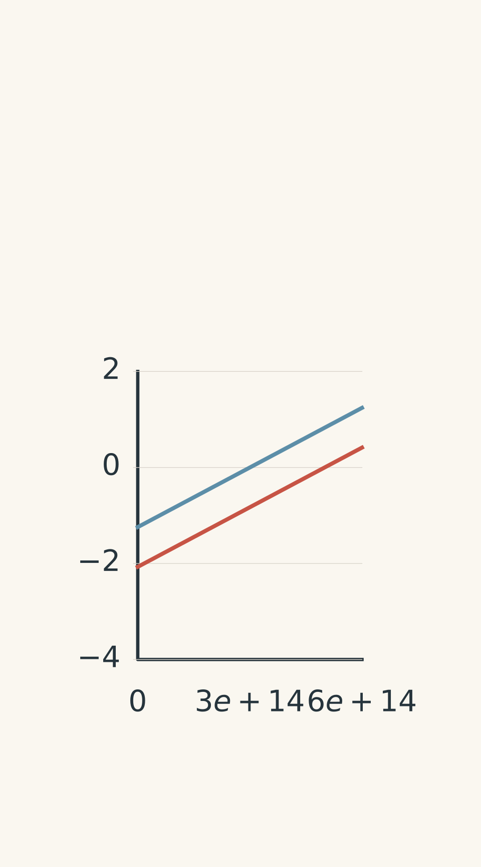
- Metal A: f₀A = 3.0 × 10¹⁴ Hz; −φA = −1.242 eV
- Metal B: f₀B = 5.0 × 10¹⁴ Hz; −φB = −2.070 eV
Notice what changes between the two metals. The gradients are equal, but the line for the metal with the larger work function has a more negative vertical intercept and a higher threshold frequency.
At the same frequency above both thresholds, that metal also produces electrons with a lower maximum kinetic energy.
03Worked example: Find Planck’s constant from a kinetic-energy graph
A metal’s maximum-kinetic-energy-versus-frequency graph passes through these two points:
- At \(f=4.0\times10^{14}\\,\text{Hz}\), \(K_{\max}=0.30\\,\text{eV}\).
- At \(f=6.0\times10^{14}\\,\text{Hz}\), \(K_{\max}=1.13\\,\text{eV}\).
Calculate Planck’s constant in SI units, the work function, and the threshold frequency.
Step 1: Calculate the gradient.
The gradient is the change in kinetic energy divided by the change in frequency:
\[ \begin{aligned} m&=\frac{\Delta K_{\max}}{\Delta f}\\\\[4pt] &=\frac{1.13-0.30}{(6.0-4.0)\times10^{14}}\\\\[4pt] &=4.15\times10^{-15}\\,\text{eV s} \end{aligned} \]
Because this is a kinetic-energy graph, the gradient gives \(h\). However, the energy is measured in electronvolts, not joules.
Step 2: Convert Planck’s constant into SI units.
Use \(1\\,\text{eV}=1.602\times10^{-19}\\,\text{J}\).
\[ \begin{aligned} h&=(4.15\times10^{-15}) (1.602\times10^{-19})\\\ &=6.65\times10^{-34}\\,\text{J s} \end{aligned} \]
This is the expected order of magnitude for Planck’s constant.
Step 3: Find the work function from the vertical intercept.
Using \(K_{\max}=hf-\phi\) at the first point,
\[ \begin{aligned} 0.30&=(4.15\times10^{-15})(4.0\times10^{14})-\phi\\\ 0.30&=1.66-\phi\\\ \phi&=1.36\\,\text{eV} \end{aligned} \]
Converting to joules,
\[ \phi=(1.36)(1.602\times10^{-19}) =2.18\times10^{-19}\\,\text{J} \]
The vertical intercept is therefore \(-1.36\\,\text{eV}\), not \(+1.36\\,\text{eV}\).
Step 4: Calculate the threshold frequency.
At threshold, \(K_{\max}=0\), so \(f_0=\phi/h\). Keep the energy units consistent by using the gradient in \(\text{eV s}\):
\[ \begin{aligned} f_0&=\frac{1.36\\,\text{eV}} {4.15\times10^{-15}\\,\text{eV s}}\\\ &=3.28\times10^{14}\\,\text{Hz} \end{aligned} \]
The threshold is below both measured frequencies, as expected. The graph tells us that the metal requires a photon frequency of at least \(3.28\times10^{14}\\,\text{Hz}\) for photoelectric emission.
02Stopping potential versus frequency
The second graph uses a different vertical quantity, but it describes the same physics.
In a photoelectric experiment, emitted electrons travel towards a collector. Applying a reverse potential opposes their motion. Increase this reverse potential until even the fastest electrons cannot reach the collector.
The magnitude of that minimum stopping potential is \(V_s\).
The maximum kinetic energy of an electron is related to the stopping potential by
\[ K_{\max}=eV_s \]
Here, \(e\) is the magnitude of the electron’s charge:
\[ e=1.602\times10^{-19}\\,\text{C} \]
The electron itself has charge \(-e\), but \(V_s\) here is defined as the positive magnitude of the stopping potential. Using \(e\) avoids introducing an unnecessary negative sign.
Substitute \(K_{\max}=eV_s\) into the photoelectric equation:
\[ eV_s=hf-\phi \]
Divide both sides by \(e\):
\[ \boxed{V_s=\frac{h}{e}f-\frac{\phi}{e}} \]
This is another straight-line equation. The crucial difference is that the vertical axis now measures potential difference rather than kinetic energy.
Measuring the stopping potential
- Photoelectric apparatus
Light → Cathode → Collector
Light ejects electrons from the metal cathode.
A voltmeter measures the reverse voltage supplied by a variable power supply.
- Stopping condition
Kₘₐₓ = eVₛ
Increase reverse voltage until the fastest electrons cannot reach the collector.
The photocurrent falls to zero in the ideal model.
What the gradient tells you
Comparing the stopping-potential equation with \(y=mx+b\) gives
\[ \boxed{\text{Gradient}=\frac{h}{e}} \]
The gradient is not Planck’s constant by itself.
If the graph’s gradient is \(m_V\), measured in volts per hertz, then
\[ \boxed{h=e\\,m_V} \]
The units explain why this works:
\[ \text{C}\times\text{V s}=\text{J s} \]
A common exam mistake is to divide the gradient by the electron charge or to forget the charge altogether. For a graph of positive stopping-potential magnitude against frequency, you must multiply the gradient by \(e\) to obtain \(h\) in \(\text{J s}\).
What the intercepts tell you
From the same equation,
\[ \boxed{y\text{-intercept}=-\frac{\phi}{e}} \]
Therefore,
\[ \boxed{\phi=-e\\,b} \]
where \(b\) is the vertical intercept in volts.
The horizontal intercept still occurs when the stopping potential is zero. Consequently,
\[ \boxed{x\text{-intercept}=f_0=\frac{\phi}{h}} \]
The threshold frequency is the same physical quantity whether you plot kinetic energy or stopping potential.
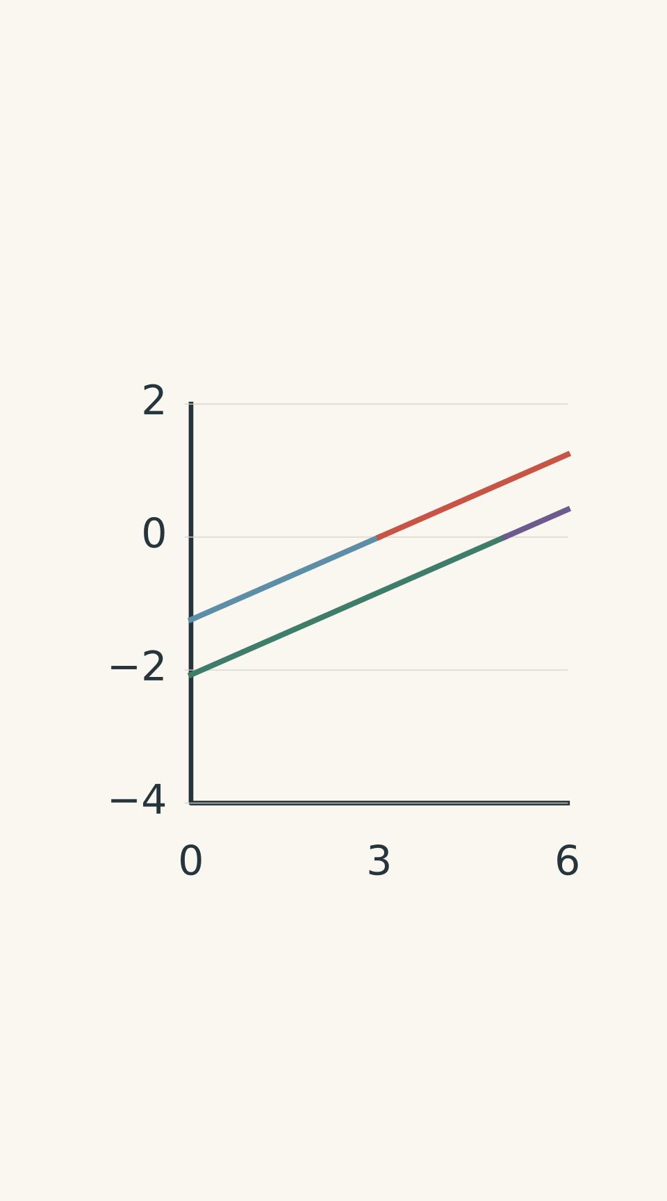
- Metal A: extrapolation below f₀A
- Metal A: physical line, f ≥ f₀A
- Metal B: extrapolation below f₀B
- Metal B: physical line, f ≥ f₀B
There is a useful shortcut when the vertical axis is in volts. The numerical value of the work function in electronvolts equals the magnitude of the vertical intercept in volts:
- A vertical intercept of \(-1.5\\,\text{V}\) corresponds to a work function of \(1.5\\,\text{eV}\).
- In joules, that work function is \(1.5\times1.602\times10^{-19}\\,\text{J}\).
This shortcut works because an electron gains one electronvolt of energy when it moves through a potential difference of one volt. The units are different, even when the numerical values match.
05Worked example: Read a stopping-potential graph with a scaled frequency axis
A stopping-potential-versus-frequency graph uses the horizontal axis \(f/(10^{14}\\,\text{Hz})\). For metal A, two points are \((5.0,0.60\\,\text{V})\) and \((7.0,1.43\\,\text{V})\).
Metal B has the same gradient, but its horizontal intercept is at a coordinate of \(4.20\).
Find Planck’s constant, both work functions, and the threshold frequency of each metal.
Step 1: Calculate the gradient, paying attention to the frequency scale.
The displayed gradient is
\[ \begin{aligned} m_{\text{displayed}} &=\frac{1.43-0.60}{7.0-5.0}\\\ &=0.415\\,\text{V per coordinate unit} \end{aligned} \]
Each horizontal coordinate unit represents \(10^{14}\\,\text{Hz}\). Therefore, the physical gradient is
\[ \begin{aligned} m_V&=\frac{0.415\\,\text{V}}{10^{14}\\,\text{Hz}}\\\ &=4.15\times10^{-15}\\,\text{V s} \end{aligned} \]
Do not use \(0.415\) directly as though the frequency axis were labelled in hertz.
Step 2: Calculate Planck’s constant.
For a stopping-potential graph, \(h=e\\,m_V\):
\[ \begin{aligned} h&=(1.602\times10^{-19}\\,\text{C})\\\ &\quad\times(4.15\times10^{-15}\\,\text{V s})\\\ &=6.65\times10^{-34}\\,\text{J s} \end{aligned} \]
The gradient is common to both metals, so the same value of \(h\) applies to each.
Step 3: Find metal A’s work function and threshold frequency.
Using the first point and the physical gradient, the vertical intercept is
\[ \begin{aligned} b_A&=V_s-m_Vf\\\ &=0.60-(4.15\times10^{-15})(5.0\times10^{14})\\\ &=-1.475\\,\text{V} \end{aligned} \]
The work function is
\[ \begin{aligned} \phi_A&=-e b_A\\\ &=(1.602\times10^{-19})(1.475)\\\ &=2.36\times10^{-19}\\,\text{J}\\\ &=1.475\\,\text{eV} \end{aligned} \]
The threshold frequency is the horizontal intercept:
\[ \begin{aligned} f_{0,A}&=-\frac{b_A}{m_V}\\\ &=\frac{1.475}{4.15\times10^{-15}}\\\ &=3.55\times10^{14}\\,\text{Hz} \end{aligned} \]
Step 4: Find metal B’s work function and threshold frequency.
The horizontal intercept coordinate is \(4.20\), so
\[ f_{0,B}=4.20\times10^{14}\\,\text{Hz} \]
Using \(\phi_B=hf_{0,B}\),
\[ \begin{aligned} \phi_B&=(6.65\times10^{-34})(4.20\times10^{14})\\\ &=2.79\times10^{-19}\\,\text{J}\\\ &\approx1.74\\,\text{eV} \end{aligned} \]
Metal B has the higher work function and threshold frequency. Its line is parallel to metal A’s line because the gradient depends on \(h\) and \(e\), not on the identity of the metal.
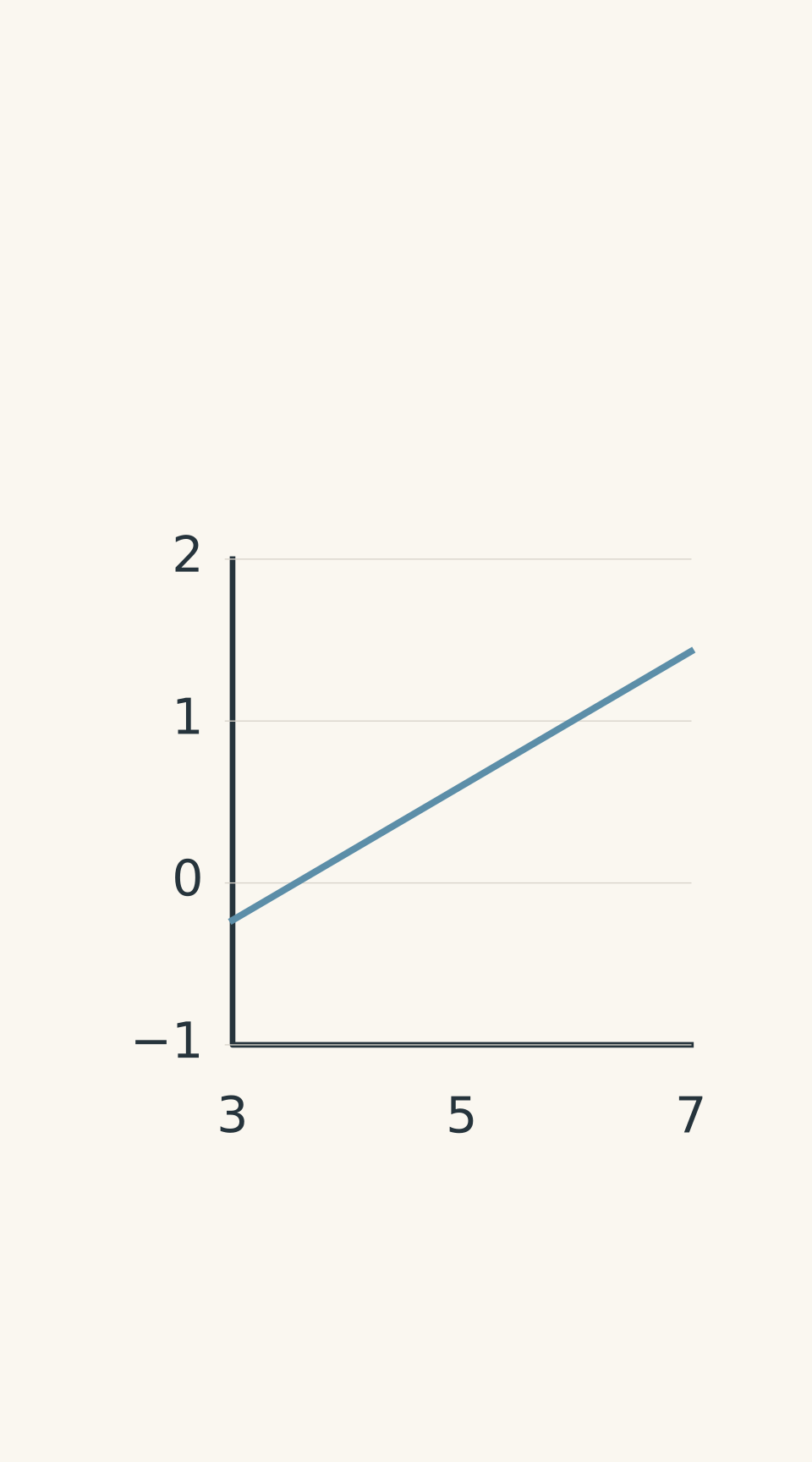
- Straight-line relation; below threshold is extrapolation
06Quick diagnostic: Common graph-reading mistakes
| Mistake | Correct interpretation |
|---|---|
| A negative vertical intercept means a negative work function. | The intercept is \(-\phi\) on a kinetic-energy graph or \(-\phi/e\) on a stopping-potential graph. The work function is positive. |
| A negative intercept means electrons have negative kinetic energy below threshold. | The line is extrapolated outside the physical region. Below \(f_0\), there is no photoelectric emission in the standard model. |
| The gradient of a stopping-potential graph is \(h\). | The gradient is \(h/e\), so calculate \(h=e\\,m_V\). |
| Use the signed electron charge \(q=-e\) and obtain a negative value of \(h\). | With \(V_s\) defined as the positive magnitude of the stopping potential, use \(e=\|q\|>0\). |
| A gradient in \(\text{eV s}\) is already in \(\text{J s}\). | Multiply by \(1.602\times10^{-19}\\,\text{J/eV}\) to convert to SI units. |
| The frequency axis is scaled by \(10^{14}\), but the displayed gradient is used unchanged. | Convert the horizontal scale first. A gradient of \(0.415\) V per coordinate unit becomes \(4.15\times10^{-15}\\,\text{V s}\). |
| Different metals must have different gradients. | Their work functions differ, shifting the lines. Their ideal gradients remain equal. |
| Increasing intensity increases the stopping potential at fixed frequency. | Intensity affects the emission rate, not the maximum kinetic energy per electron in the standard single-photon model. |
07Questions and solutions
Question 1
A maximum-kinetic-energy-versus-frequency graph has a gradient of \(4.00\times10^{-15}\\,\text{eV s}\) and a horizontal intercept of \(4.50\times10^{14}\\,\text{Hz}\).
Calculate Planck’s constant in \(\text{J s}\) and the work function in both electronvolts and joules.
Solution 1
Planck’s constant is \(6.41\times10^{-34}\\,\text{J s}\), and the work function is \(1.80\\,\text{eV}\), or \(2.88\times10^{-19}\\,\text{J}\).
The gradient of a kinetic-energy graph gives \(h\). Convert it into SI units:
\[ \begin{aligned} h&=(4.00\times10^{-15})(1.602\times10^{-19})\\\ &=6.41\times10^{-34}\\,\text{J s} \end{aligned} \]
At the horizontal intercept, \(K_{\max}=0\), so \(\phi=hf_0\). Using the gradient in \(\text{eV s}\),
\[ \begin{aligned} \phi&=(4.00\times10^{-15})(4.50\times10^{14})\\\ &=1.80\\,\text{eV} \end{aligned} \]
Convert the work function to joules:
\[ \phi=(1.80)(1.602\times10^{-19}) =2.88\times10^{-19}\\,\text{J} \]
The horizontal intercept determines the threshold frequency, while the gradient determines Planck’s constant. They provide different information about the same metal.
Question 2
At the same light frequency, which is above both metals’ thresholds, metal A has a stopping potential of \(1.40\\,\text{V}\), while metal B has a stopping potential of \(0.65\\,\text{V}\).
Calculate \(\phi_B-\phi_A\) in electronvolts and joules. Which metal has the higher threshold frequency? Explain why you do not need to know the light frequency.
Solution 2
Metal B has a work function greater than metal A’s by \(0.75\\,\text{eV}\), or \(1.20\times10^{-19}\\,\text{J}\). Metal B therefore has the higher threshold frequency.
For each metal,
\[ eV_{s,A}=hf-\phi_A \]
\[ eV_{s,B}=hf-\phi_B \]
Subtract the equations. Because both metals are illuminated at the same frequency, the \(hf\) terms cancel:
\[ e(V_{s,A}-V_{s,B})=\phi_B-\phi_A \]
Substitute the stopping potentials:
\[ \begin{aligned} \phi_B-\phi_A &=e(1.40-0.65)\\\ &=e(0.75\\,\text{V})\\\ &=0.75\\,\text{eV} \end{aligned} \]
In joules,
\[ \begin{aligned} \phi_B-\phi_A &=(1.602\times10^{-19})(0.75)\\\ &=1.20\times10^{-19}\\,\text{J} \end{aligned} \]
Since \(f_0=\phi/h\), the metal with the larger work function also has the larger threshold frequency. The unknown light frequency is irrelevant because it cancels when the two equations are subtracted.
Question 3
Two metals have parallel maximum-kinetic-energy-versus-frequency graphs. Their common gradient is \(4.14\times10^{-15}\\,\text{eV s}\).
Metal A has a threshold frequency of \(4.0\times10^{14}\\,\text{Hz}\), and metal B has a threshold frequency of \(5.5\times10^{14}\\,\text{Hz}\).
Calculate:
- the work function of each metal in electronvolts;
- the maximum kinetic energy of emitted electrons from each metal when the light frequency is \(6.0\times10^{14}\\,\text{Hz}\); and
- which metal emits electrons when the frequency is \(4.8\times10^{14}\\,\text{Hz}\).
Solution 3
Metal A has a work function of \(1.656\\,\text{eV}\), while metal B has a work function of \(2.277\\,\text{eV}\). At \(6.0\times10^{14}\\,\text{Hz}\), their maximum kinetic energies are \(0.828\\,\text{eV}\) and \(0.207\\,\text{eV}\), respectively. At \(4.8\times10^{14}\\,\text{Hz}\), only metal A emits electrons.
The gradient is \(h=4.14\times10^{-15}\\,\text{eV s}\). At threshold, \(\phi=hf_0\).
For metal A,
\[ \begin{aligned} \phi_A&=(4.14\times10^{-15})(4.0\times10^{14})\\\ &=1.656\\,\text{eV} \end{aligned} \]
For metal B,
\[ \begin{aligned} \phi_B&=(4.14\times10^{-15})(5.5\times10^{14})\\\ &=2.277\\,\text{eV} \end{aligned} \]
At \(f=6.0\times10^{14}\\,\text{Hz}\), use \(K_{\max}=h(f-f_0)\).
For metal A,
\[ \begin{aligned} K_{\max,A} &=(4.14\times10^{-15})(2.0\times10^{14})\\\ &=0.828\\,\text{eV} \end{aligned} \]
For metal B,
\[ \begin{aligned} K_{\max,B} &=(4.14\times10^{-15})(0.5\times10^{14})\\\ &=0.207\\,\text{eV} \end{aligned} \]
The same gradient does not mean the electrons have the same kinetic energy at a given frequency. Metal B has the larger work function, so less photon energy remains as kinetic energy.
Finally, \(4.8\times10^{14}\\,\text{Hz}\) is above metal A’s threshold but below metal B’s. Metal A emits electrons, while metal B does not. Below threshold, the extrapolated line must not be interpreted as a physical negative kinetic energy.
Question 4
A stopping-potential-versus-frequency graph has a gradient of \(4.12\times10^{-15}\\,\text{V s}\) and a vertical intercept of \(-1.70\\,\text{V}\).
A student claims that the threshold frequency is \(1.70\times10^{14}\\,\text{Hz}\), and that tripling the intensity of the light will triple the stopping potential.
Calculate Planck’s constant, the work function, and the correct threshold frequency. Explain both errors.
Solution 4
Planck’s constant is \(6.60\times10^{-34}\\,\text{J s}\), the work function is \(1.70\\,\text{eV}\), or \(2.72\times10^{-19}\\,\text{J}\), and the threshold frequency is \(4.13\times10^{14}\\,\text{Hz}\). The student’s threshold and intensity claims are both incorrect.
The stopping-potential gradient is \(m_V=h/e\), so
\[ \begin{aligned} h&=e\\,m_V\\\ &=(1.602\times10^{-19})(4.12\times10^{-15})\\\ &=6.60\times10^{-34}\\,\text{J s} \end{aligned} \]
The work function comes from the vertical intercept \(b=-\phi/e\):
\[ \begin{aligned} \phi&=-eb\\\ &=(1.602\times10^{-19})(1.70)\\\ &=2.72\times10^{-19}\\,\text{J}\\\ &=1.70\\,\text{eV} \end{aligned} \]
The threshold frequency is the horizontal intercept, not the magnitude of the vertical intercept:
\[ \begin{aligned} f_0&=-\frac{b}{m_V}\\\ &=\frac{1.70}{4.12\times10^{-15}}\\\ &=4.13\times10^{14}\\,\text{Hz} \end{aligned} \]
The student’s first mistake is confusing the two intercepts. The vertical intercept gives information about the work function; the horizontal intercept gives the threshold frequency.
The second mistake is confusing intensity with photon energy. At fixed frequency, tripling the intensity increases the number of incident photons per second. It can increase the photocurrent, but it does not triple the maximum kinetic energy or stopping potential in the standard single-photon model.
Question 5
An experimental graph has lost its vertical-axis label. The horizontal axis is frequency in hertz, and the vertical quantity is known to be either maximum kinetic energy in electronvolts or stopping potential in volts.
Two parallel lines represent metals A and B. Their gradients are numerically \(4.14\times10^{-15}\) in the appropriate units per hertz, and their horizontal intercepts are:
- Metal A: \(4.0\times10^{14}\\,\text{Hz}\)
- Metal B: \(5.5\times10^{14}\\,\text{Hz}\)
At \(6.0\times10^{14}\\,\text{Hz}\), their vertical readings are \(0.83\) and \(0.21\), respectively.
Two students make competing claims:
- Student 1 says the graph must be a kinetic-energy graph because a stopping potential cannot have a negative vertical intercept.
- Student 2 says that metal B will emit electrons at \(4.8\times10^{14}\\,\text{Hz}\) if the light intensity is made sufficiently high.
Assume the standard HSC single-photon model, and define stopping potential as a positive magnitude.
Determine whether the vertical axis can be identified from the graph alone. Calculate Planck’s constant and both work functions, decide which metals emit at \(4.8\times10^{14}\\,\text{Hz}\), and assess both students’ claims.
Solution 5
Neither student is correct. The graph alone cannot identify the vertical quantity, and metal B will not emit electrons at \(4.8\times10^{14}\\,\text{Hz}\), regardless of intensity within the stated model. Planck’s constant is approximately \(6.63\times10^{-34}\\,\text{J s}\), while the work functions are \(1.656\\,\text{eV}\) for A and \(2.277\\,\text{eV}\) for B.
First, identify what the gradient means.
If the graph plots maximum kinetic energy in electronvolts, its gradient gives \(h\) in \(\text{eV s}\). Converting to SI units,
\[ \begin{aligned} h&=(4.14\times10^{-15})(1.602\times10^{-19})\\\ &=6.63\times10^{-34}\\,\text{J s} \end{aligned} \]
If the graph plots stopping potential in volts, the gradient gives \(h/e\). Multiplying by the elementary charge gives
\[ \begin{aligned} h&=(1.602\times10^{-19})(4.14\times10^{-15})\\\ &=6.63\times10^{-34}\\,\text{J s} \end{aligned} \]
Both interpretations give the same physical constant.
Second, calculate the work functions.
The horizontal intercept gives the threshold frequency, so \(\phi=hf_0\).
For metal A,
\[ \begin{aligned} \phi_A&=(4.14\times10^{-15})(4.0\times10^{14})\\\ &=1.656\\,\text{eV}\\\ &=2.65\times10^{-19}\\,\text{J} \end{aligned} \]
For metal B,
\[ \begin{aligned} \phi_B&=(4.14\times10^{-15})(5.5\times10^{14})\\\ &=2.277\\,\text{eV}\\\ &=3.65\times10^{-19}\\,\text{J} \end{aligned} \]
Metal B has the higher work function, which explains its higher threshold frequency.
Third, decide whether the vertical axis can be identified.
No. For an emitted electron, \(K_{\max}=eV_s\). When kinetic energy is expressed in electronvolts and stopping potential in volts, their numerical values are equal:
\[ K_{\max}\text{ in eV}=V_s\text{ in V} \]
For example, a kinetic energy of \(0.83\\,\text{eV}\) corresponds to a stopping potential of \(0.83\\,\text{V}\). The same numerical line can therefore represent either quantity. An axis label or an independent measurement is needed to distinguish them.
Student 1’s argument also fails because the negative vertical intercept is an extrapolation to zero frequency. It is not a physical measurement of negative kinetic energy or a negative stopping-potential magnitude. Both graph types have negative extrapolated vertical intercepts.
Finally, test the intensity claim at \(4.8\times10^{14}\\,\text{Hz}\).
Metal A’s threshold is \(4.0\times10^{14}\\,\text{Hz}\), so it emits electrons. Its maximum kinetic energy is
\[ \begin{aligned} K_{\max,A} &=(4.14\times10^{-15}) (4.8-4.0)\times10^{14}\\\ &=0.331\\,\text{eV} \end{aligned} \]
If the graph is a stopping-potential graph, this corresponds to \(V_{s,A}=0.331\\,\text{V}\).
Metal B’s threshold is \(5.5\times10^{14}\\,\text{Hz}\), so the incident photons do not have enough energy to release electrons. Increasing intensity supplies more photons, but each photon still has insufficient energy. Metal B therefore does not emit electrons under the stated conditions.
The tempting mistake is to treat intensity as though it increases the energy of each photon. It does not. The threshold condition depends on frequency, while intensity controls the number of photons arriving per second.
Once you can read the gradient and intercepts reliably, the next useful connection is a photocurrent-versus-intensity graph. Together, the graphs show how frequency determines the maximum energy of emitted electrons, while intensity determines how many electrons can be emitted per second.