
How to Read an AAS Calibration Curve in HSC Chemistry
Learn how to use AAS calibration curves to determine unknown concentrations, check blanks and calibrated ranges, and correct for dilution factors. Includes worked examples, common mistakes, and challenging HSC-style questions with detailed solutions.
Suppose an atomic absorption spectroscopy (AAS) instrument gives an unknown sample an absorbance of 0.250. Does that mean its concentration is 0.250 mg/L? No. Absorbance is the instrument’s response, not the concentration itself.
Now suppose standards at 4.0 mg/L and 6.0 mg/L give absorbances of 0.201 and 0.300, respectively. The unknown sits about halfway between these readings, so its concentration is close to 5.0 mg/L. But what if its absorbance is higher than every standard? Extending the line might produce a number, but that doesn’t mean the number is reliable.
Reading an AAS calibration curve is about making three decisions correctly: finding the concentration supported by the standards, checking that the measurement is within the calibrated range, and correcting for any dilution before reporting the original sample’s concentration.
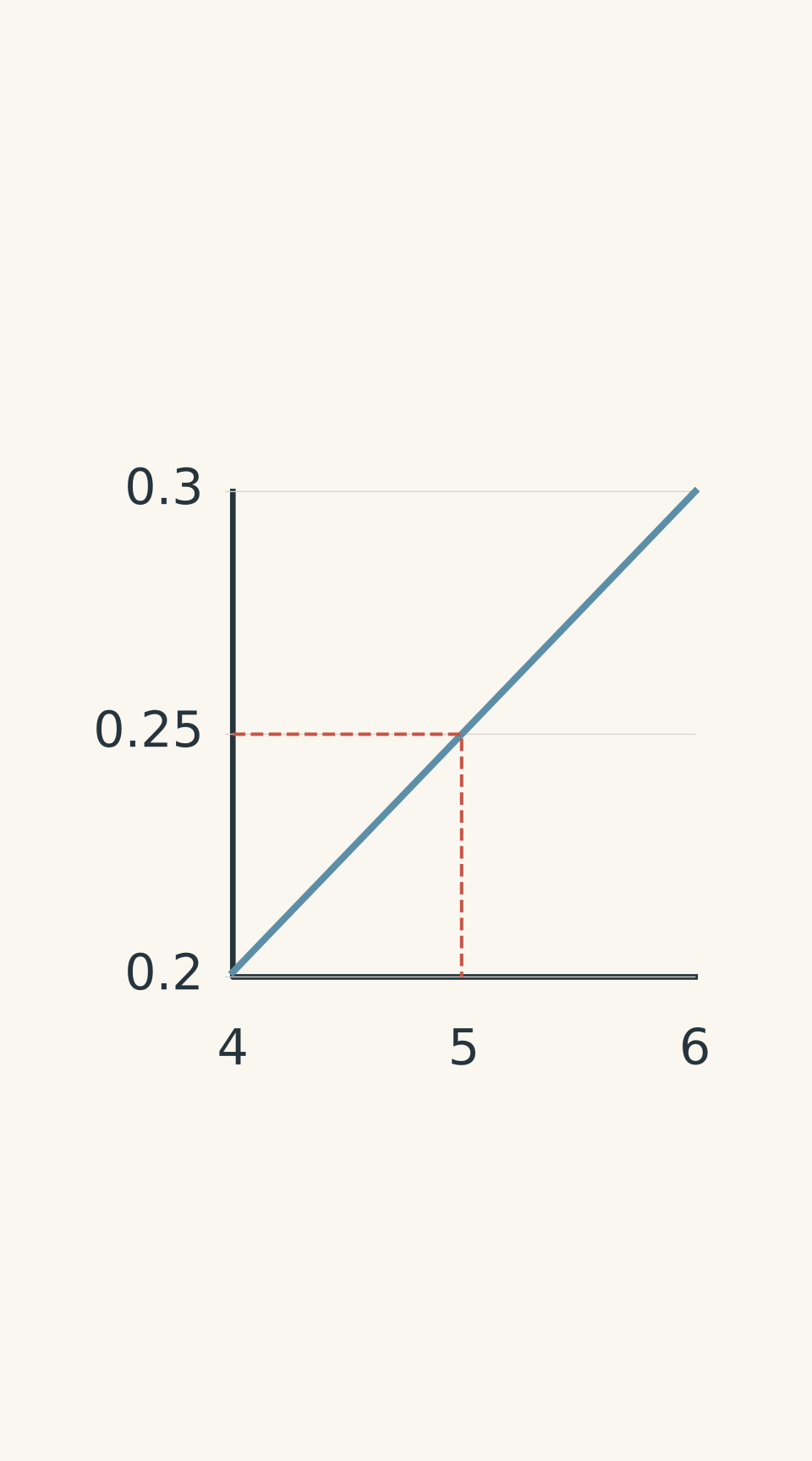
- Calibration standards
- Unknown: A = 0.250 → ≈5.0 mg/L
01Quick decision rule
Use this sequence whenever an AAS question gives you a calibration curve, an equation, or a set of standards.
- Check the axes and units. For the usual calibration plot, concentration is on the horizontal axis and absorbance is on the vertical axis.
- Check the blank. Confirm that the standards and unknown have been measured and corrected in the same way.
- Check the range. If the unknown’s absorbance falls within the responses covered by the standards, use interpolation. If it falls outside, do not rely on extrapolation.
- Find the concentration. Read it from the graph or calculate it using the calibration equation, if the relationship is adequately linear.
- Correct for dilution. Multiply the measured concentration by the total dilution factor.
- Report the original concentration with units. Make it clear whether the result refers to the diluted solution or the original sample.
The key distinction is simple: the calibration curve gives you the concentration of the solution that entered the instrument. You must account for any preparation steps to recover the concentration in the original sample.
02What an AAS calibration curve actually tells you
How AAS produces a measurement
Atomic absorption spectroscopy measures how much light is absorbed by atoms of a particular element.
An element-specific light source sends light through a sample that has been atomised. In flame AAS, the flame converts the sample into free atoms. Atoms of the target element absorb some of the light at characteristic wavelengths, and a detector measures the transmitted light.
More target atoms in the light path generally produce greater absorbance, provided the instrument is operating within a suitable range and the sample is introduced consistently.
How flame AAS measures absorption
- Element-specific lamp
Emits characteristic-wavelength light (I₀).
- Flame with atomised sample
Target atoms absorb some incident light.
- Detector
Measures weaker transmitted light (I < I₀).
Absorbance, \(A\), can be expressed as
\[
A=\log_{10}\left(\frac{I_0}{I}\right)
\]
where:
- \(A\) is absorbance, which is dimensionless.
- \(I_0\) is the intensity of light entering the atom cloud.
- \(I\) is the intensity of light transmitted through it.
A larger difference between the incoming and transmitted light corresponds to greater absorbance.
However, absorbance is not automatically equal to concentration. You need a calibration relationship to translate one into the other.
How standards establish the relationship
A calibration standard is a solution containing a known concentration of the element being measured.
For example, a chemist might prepare standards containing 0, 2.0, 4.0, 6.0, and 8.0 mg/L of copper. Each standard is measured using the same AAS settings, wavelength, and atomisation conditions.
The chemist then plots the known concentrations against their measured absorbances.
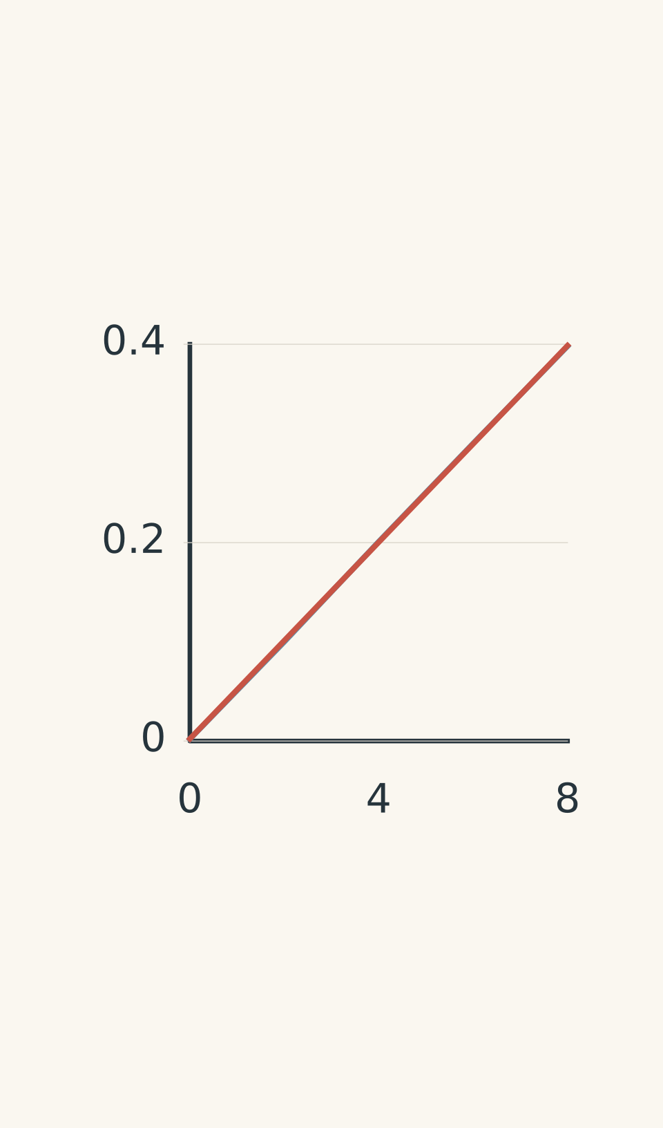
- Measured standards (schematic)
- Linear best fit
The resulting graph is the calibration curve. It provides an experimentally established relationship between concentration and instrument response.
Within a suitable working range, this relationship is often approximately linear. The points may not fall perfectly on a straight line because measurements have uncertainty.
Use the line of best fit rather than joining each point with a zigzag line. The purpose is to estimate the overall relationship, not reproduce every small measurement variation.
The calibration equation
If the calibration relationship is linear, it can be written as
\[
A=mc+b
\]
where:
- \(A\) is absorbance.
- \(c\) is concentration, such as in mg/L.
- \(m\) is the slope of the calibration line.
- \(b\) is the vertical intercept, or the predicted absorbance when \(c=0\).
If concentration is measured in mg/L, the slope has units of L/mg. The intercept has the same units as absorbance.
The slope describes the instrument’s sensitivity over the calibrated range. A steeper slope means that a given increase in concentration produces a larger increase in absorbance.
To calculate an unknown concentration, rearrange the equation:
\[
\boxed{c=\frac{A-b}{m}}
\]
Subtract the intercept from the measured absorbance first, then divide by the slope.
Do not automatically assume that \(b=0\). A non-zero intercept can arise from the fitted calibration data or the way the readings were processed. Use the equation provided unless you have a justified reason to use a different model.
This equation also has a limitation: it assumes a linear calibration relationship. If the graph is visibly curved, a straight-line equation may not be appropriate across the whole range.
03Check the axes and blank before reading the curve
1. Read the axis labels
For the usual AAS calibration graph:
- The horizontal axis shows the known concentration of each standard, including its units.
- The vertical axis shows the measured absorbance.
Suppose an unknown has an absorbance of 0.30. You start at 0.30 on the vertical axis, move across to the calibration line, and then move down to the horizontal axis to read the concentration.
Do not read concentration directly from the absorbance axis. The two quantities are related, but they are not interchangeable.
Also check that the calibration applies to the correct element and measurement conditions. A calibration curve for copper cannot be used to determine zinc concentration.
2. Understand the blank
A blank contains the solvent and relevant reagents but no analyte, meaning the element whose concentration you want to measure.
For example, if copper standards are prepared in dilute nitric acid, the blank would generally contain the same acid matrix without the copper.
The blank helps establish the background response from the solvent and reagents. The instrument may use it to set a zero baseline, or the blank may be subtracted from measured readings.
The important point is consistency.
Prepare and measure AAS solutions consistently
| Reagent blank | Solvent and reagents; no analyte. |
|---|---|
| Calibration standards | Analyte present at known concentrations. |
| Unknown sample | Analyte present at an unknown concentration. |
If the standards were blank-corrected, the unknown must be treated consistently. If the calibration equation was fitted to raw readings and already includes the blank response in its intercept, do not subtract that blank from the unknown and then use the uncorrected equation.
That would count the background correction twice.
A blank also cannot automatically correct every matrix effect. Differences in acidity, dissolved salts, or other sample components may affect atomisation or absorption. Standards should have a sufficiently similar matrix to the unknown, or an appropriate correction method must be used.
04How to read a concentration from the curve
If the unknown’s absorbance falls within the calibrated range, use interpolation.
Interpolation means estimating a value between known data points or within the range covered by the calibration model. It is supported by measurements on either side of the unknown response.
Follow these steps:
- Locate the unknown absorbance on the vertical axis.
- Move horizontally until you reach the calibration line.
- Move vertically down to the concentration axis.
- Read the corresponding concentration, including its units.
- Check that the result is consistent with the positions of the surrounding standards.
- Standards: (4.0, 0.201) and (6.0, 0.300)
- Unknown A = 0.250; estimated c ≈ 5.0 mg/L
If you have two neighbouring standards and a straight-line relationship, you can calculate the estimate more precisely.
Let the standards have concentrations \(c_1\) and \(c_2\), with absorbances \(A_1\) and \(A_2\). If the unknown has absorbance \(A_x\), then
\[
c_x=c_1+
\frac{A_x-A_1}{A_2-A_1}(c_2-c_1)
\]
This calculates how far the unknown lies between the two absorbance readings, then applies the same fraction to the concentration interval.
Worked example: Estimate an unknown concentration from a graph
Question: A linear AAS calibration curve gives an absorbance of 0.201 at 4.0 mg/L and 0.300 at 6.0 mg/L. An unknown sample has an absorbance of 0.250. The calibrated range is 0-8.0 mg/L. Estimate the unknown concentration.
Step 1
The unknown absorbance of 0.250 lies between 0.201 and 0.300. Therefore, interpolation is appropriate.
Step 2
\[
\begin{aligned}
f&=\frac{0.250-0.201}{0.300-0.201}\\
&=\frac{0.049}{0.099}\\
&=0.495
\end{aligned}
\]
The unknown lies about 49.5% of the way from the first standard to the second.
Step 3
\[
\begin{aligned}
c_x&=4.0+0.495(6.0-4.0)\\
&=4.99\ \mathrm{mg\,L^{-1}}\\
&\approx 5.0\ \mathrm{mg\,L^{-1}}
\end{aligned}
\]
Answer: The estimated concentration is \(5.0\ \mathrm{mg\,L^{-1}}\).
Step 4
The answer lies between 4.0 and 6.0 mg/L, as it should. The unknown absorbance is also approximately halfway between the two standard readings.
The result is consistent with the calibration curve.
05How to apply a dilution factor
A calibration curve determines the concentration of the solution measured by the instrument. If the original sample was diluted before measurement, that is not yet the final answer.
Suppose you transfer 5.00 mL of an original sample into a volumetric flask and add solvent until the total volume is 50.0 mL. The original sample has been diluted tenfold.
The dilution factor is
\[
DF=\frac{V_f}{V_a}
\]
where:
- \(DF\) is the dilution factor.
- \(V_f\) is the final volume of the diluted solution.
- \(V_a\) is the volume of the original sample transferred into the flask.
Both volumes must use the same units.
The original concentration is then
\[
c_{\mathrm{original}}=c_{\mathrm{diluted}}\times DF
\]
Tenfold dilution
- Transfer aliquot
Pipette 5.00 mL of original sample.
- Dilute to the mark
Add solvent until final volume is 50.0 mL.
- Diluted solution
Concentration is one-tenth of the original.
Notice that the formula uses the final volume, not the volume of solvent added. If you add 45.0 mL of solvent to 5.00 mL of sample, the final volume is 50.0 mL, giving a dilution factor of 10.0.
If the sample undergoes multiple dilutions, multiply the individual dilution factors to obtain the total factor.
For example, a tenfold dilution followed by a fivefold dilution gives
\[
DF_{\mathrm{total}}=10.0\times5.0=50.0
\]
Worked example: Calculate the original concentration after dilution
Question: An AAS calibration equation is
\[
A=(0.0420\ \mathrm{L\,mg^{-1}})c+0.006
\]
The calibration range is 0-10.0 mg/L. A 5.00 mL aliquot of an unknown sample is diluted to a final volume of 50.0 mL. The diluted solution gives an absorbance of 0.258. Calculate the concentration in the original sample.
Step 1
The measured absorbance is 0.258, and the calibration equation includes an intercept of 0.006.
Rearrange the equation:
\[
c_{\mathrm{diluted}}=\frac{A-b}{m}
\]
Step 2
\[
\begin{aligned}
c_{\mathrm{diluted}}
&=\frac{0.258-0.006}
{0.0420\ \mathrm{L\,mg^{-1}}}\\
&=\frac{0.252}{0.0420\ \mathrm{L\,mg^{-1}}}\\
&=6.00\ \mathrm{mg\,L^{-1}}
\end{aligned}
\]
The diluted sample contains 6.00 mg/L of the analyte. This is within the calibrated range of 0-10.0 mg/L.
Step 3
\[
\begin{aligned}
DF&=\frac{V_f}{V_a}\\
&=\frac{50.0\ \mathrm{mL}}{5.00\ \mathrm{mL}}\\
&=10.0
\end{aligned}
\]
Step 4
\[
\begin{aligned}
c_{\mathrm{original}}
&=c_{\mathrm{diluted}}\times DF\\
&=6.00\ \mathrm{mg\,L^{-1}}\times10.0\\
&=60.0\ \mathrm{mg\,L^{-1}}
\end{aligned}
\]
Answer: The original sample concentration is \(60.0\ \mathrm{mg\,L^{-1}}\).
The important check is that the solution measured by the instrument had a concentration of 6.00 mg/L, which falls within the calibrated range. The original sample can have a concentration greater than the highest standard because it was diluted before measurement.
06Why extrapolation is unreliable
Interpolation and extrapolation may look similar on a graph, but they have different levels of support.
- Interpolation estimates a concentration within the range covered by the standards.
- Extrapolation extends the calibration relationship beyond that range.
Suppose your highest standard has a concentration of 8.0 mg/L and an absorbance of 0.40. Your unknown has an absorbance of 0.52.
Extending the calibration line might suggest a concentration of around 10 mg/L. But the standards have not demonstrated that the relationship remains linear at that higher concentration.
At high concentrations, the instrument’s response may depart from linearity. At very low concentrations, background signals and measurement noise may become important relative to the analyte signal. Matrix effects can also change the response.
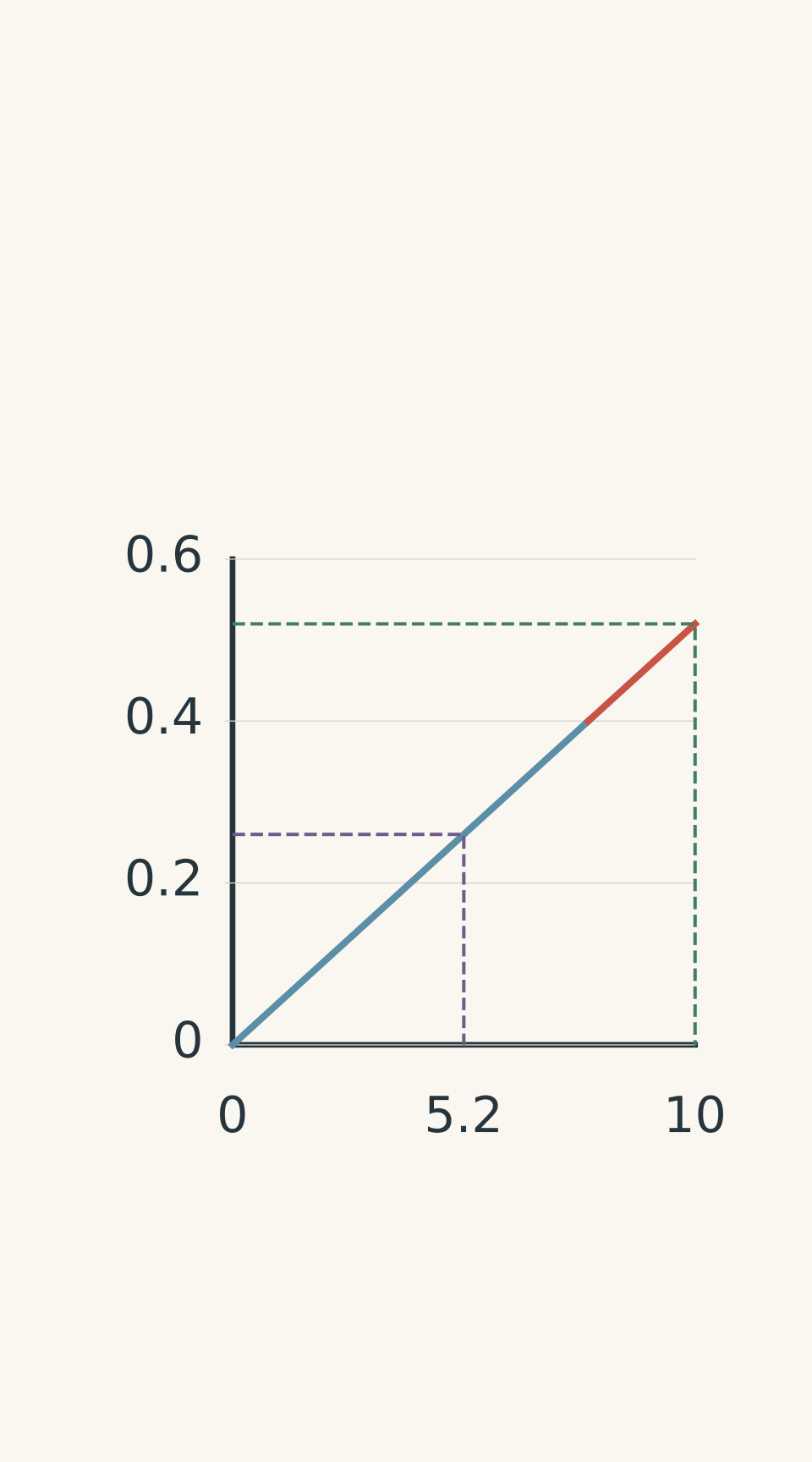
- Calibration standards and line
- Extrapolation beyond range (unreliable)
- Before dilution: A = 0.52; extrapolated c ≈ 10.4 mg/L, unreliable
- After twofold dilution: A = 0.26; measured c ≈ 5.2 mg/L
For an unknown above the calibrated range, the better approach is to dilute the sample by a known factor and measure it again. The diluted reading can then be used to determine the concentration within the established range.
For an unknown below the usable range, prepare lower-concentration standards and recalibrate, or use a suitable more sensitive method. A signal near the blank may not support a reliable quantitative result, even if an equation produces a small positive concentration.
The general rule is that an equation can return a number outside its validated range, but the calculation alone does not establish that the number is reliable.
07AAS versus a qualitative flame test
Both techniques involve light and atoms, but they measure different things.
| Feature | Atomic absorption spectroscopy (AAS) | Flame test |
|---|---|---|
| Signal observed | Absorption of element-specific lamp light | Light emitted by excited species in a flame |
| Main purpose | Quantitative analysis after calibration | Qualitative identification of possible metal ions |
| How the result is interpreted | Absorbance is related to concentration using standards | Flame colour is compared with characteristic colours |
| Main limitation | Requires suitable calibration, range, and control of interferences | Colour does not provide a reliable concentration and may be affected by mixtures or contamination |
In a flame test, heat excites atoms or ions. As they return to lower-energy states, they emit light at characteristic wavelengths. A blue-green flame, for example, may be consistent with copper.
In AAS, an external light source sends characteristic light through atomised sample. The instrument measures how much of that light is absorbed.
Flame test versus flame AAS
| Flame test | Heated sample emits characteristic coloured light. Qualitative identification; colour does not reliably quantify concentration. |
|---|---|
| Flame AAS | Element-specific lamp light passes through atomised sample to a detector; target atoms absorb light. Quantitative measurement using a calibration curve. |
A flame test can suggest which metal ion is present, but it cannot establish that a solution contains 5.0 mg/L rather than 10.0 mg/L. The intensity of a flame colour is not a reliable concentration scale.
AAS can determine concentration because its response is compared with standards of known concentration. However, AAS is not automatically reliable just because an instrument produces a numerical reading. The calibration and sample preparation still need to be appropriate.
One final distinction is worth remembering: a flame may be used to atomise a sample in flame AAS, but the instrument measures absorption of lamp light, not the visible colour of the flame.
08Common mistakes
Reading concentration from the vertical axis. Absorbance is the instrument response, while concentration is the quantity being determined. For the usual calibration graph, read across from absorbance and down to concentration.
Forgetting the intercept. If the calibration equation is \(A=mc+b\), dividing \(A\) by \(m\) ignores the intercept. Use \(c=(A-b)/m\).
Subtracting the blank twice. If the fitted equation already includes the blank response, subtracting the blank from the unknown without adjusting the equation makes the result inconsistent. Treat standards and unknowns in the same way.
Extrapolating beyond the standards. A mathematically calculated concentration is not necessarily a valid measurement. Dilute a high-concentration sample and remeasure it within the calibrated range.
Forgetting the dilution factor. The calibration curve gives the concentration of the diluted solution, not automatically the original sample. Multiply by the total dilution factor.
Using the volume of solvent added. The dilution factor uses the final solution volume divided by the original aliquot volume, not the solvent volume divided by the aliquot volume.
Treating a flame test as quantitative. Flame colour may help identify an element, but concentration must be determined using an appropriate quantitative method.
09Questions and solutions
Question 1
A set of copper standards gives the following results.
| Concentration (mg/L) | Absorbance |
|---|---|
| 0.0 | 0.00 |
| 2.0 | 0.08 |
| 4.0 | 0.16 |
| 6.0 | 0.24 |
An unknown sample has an absorbance of 0.20. Assuming the calibration is linear across this range, estimate its copper concentration.
Solution 1
The estimated copper concentration is \(5.0\ \mathrm{mg\,L^{-1}}\). The unknown absorbance lies halfway between the readings for 4.0 and 6.0 mg/L, so its concentration should also lie halfway between those standards.
Using linear interpolation,
\[
\begin{aligned}
c&=4.0+
\frac{0.20-0.16}{0.24-0.16}(6.0-4.0)\\
&=4.0+\frac{0.04}{0.08}(2.0)\\
&=5.0\ \mathrm{mg\,L^{-1}}
\end{aligned}
\]
The result is within the calibrated range, so interpolation is appropriate.
Question 2
An AAS calibration equation for an element is
\[
A=(0.0400\ \mathrm{L\,mg^{-1}})c+0.0020
\]
The calibrated range is 0-8.00 mg/L.
A 2.00 mL aliquot of an original sample is diluted to 20.00 mL. Then, 5.00 mL of this first diluted solution is transferred into another volumetric flask and diluted to a final volume of 25.00 mL.
The final solution has an absorbance of 0.0660.
Calculate the concentration in the original sample and explain why the dilution factor must be applied twice.
Solution 2
The original sample concentration is \(80.0\ \mathrm{mg\,L^{-1}}\). The sample underwent two successive dilutions, so both dilution factors must be included.
First, calculate the concentration of the final solution using the calibration equation.
\[
\begin{aligned}
c_{\mathrm{final}}
&=\frac{A-b}{m}\\
&=\frac{0.0660-0.0020}
{0.0400\ \mathrm{L\,mg^{-1}}}\\
&=1.60\ \mathrm{mg\,L^{-1}}
\end{aligned}
\]
This concentration is within the calibrated range.
Next, calculate each dilution factor:
\[
DF_1=\frac{20.00}{2.00}=10.0
\]
\[
DF_2=\frac{25.00}{5.00}=5.00
\]
The total dilution factor is
\[
DF_{\mathrm{total}}=10.0\times5.00=50.0
\]
Therefore,
\[
\begin{aligned}
c_{\mathrm{original}}
&=1.60\ \mathrm{mg\,L^{-1}}\times50.0\\
&=80.0\ \mathrm{mg\,L^{-1}}
\end{aligned}
\]
The concentration of the final solution is only 1.60 mg/L, but the original sample was 50 times more concentrated. Applying only one dilution factor would underestimate the original concentration.
Question 3
An AAS calibration equation is
\[
A=(0.0480\ \mathrm{L\,mg^{-1}})c+0.0060
\]
The standards cover concentrations from 0 to 8.0 mg/L. An undiluted unknown sample gives an absorbance of 0.510.
A student substitutes this value into the equation and calculates a concentration of 10.5 mg/L.
The student then dilutes the sample twofold and obtains an absorbance of 0.258.
Determine the concentration that should be reported. Explain why the second measurement provides stronger evidence, even if both calculations give the same final answer.
Solution 3
The concentration to report is \(10.5\ \mathrm{mg\,L^{-1}}\), based on the diluted measurement. The initial extrapolation is not a reliable basis for the result because the undiluted sample’s absorbance lies outside the calibrated range.
The highest standard has a predicted absorbance of
\[
\begin{aligned}
A_{\max}
&=0.0480(8.0)+0.0060\\
&=0.390
\end{aligned}
\]
The original absorbance of 0.510 is greater than 0.390. Therefore, the original reading is outside the range tested by the standards.
For the twofold-diluted sample,
\[
\begin{aligned}
c_{\mathrm{diluted}}
&=\frac{0.258-0.0060}
{0.0480\ \mathrm{L\,mg^{-1}}}\\
&=5.25\ \mathrm{mg\,L^{-1}}
\end{aligned}
\]
This is within the calibrated range of 0-8.0 mg/L.
Correcting for the twofold dilution gives
\[
\begin{aligned}
c_{\mathrm{original}}
&=5.25\ \mathrm{mg\,L^{-1}}\times2.00\\
&=10.5\ \mathrm{mg\,L^{-1}}
\end{aligned}
\]
The two calculations happen to agree numerically. However, the first uses the calibration relationship beyond the range supported by the standards, while the second uses a measurement within that range. Agreement does not make extrapolation valid; the in-range measurement is the defensible basis for the reported result.
Question 4
A copper calibration curve was fitted using raw, unblank-corrected readings:
\[
A=0.0200c+0.0300
\]
Here, \(c\) is the copper concentration in mg/L. The reagent blank has a raw absorbance of 0.0300, and an unknown copper sample has a raw absorbance of 0.170.
Calculate the copper concentration. Explain why subtracting the blank from the unknown and then using the original equation would give an incorrect result. Would a blue-green flame test provide an equivalent quantitative measurement?
Solution 4
The copper concentration is \(7.00\ \mathrm{mg\,L^{-1}}\). The raw unknown reading must be used directly with the raw calibration equation because the blank response is already represented by its intercept.
Rearrange the equation:
\[
c=\frac{A-b}{m}
\]
Substitute the raw absorbance:
\[
\begin{aligned}
c&=\frac{0.170-0.0300}{0.0200}\\
&=\frac{0.140}{0.0200}\\
&=7.00\ \mathrm{mg\,L^{-1}}
\end{aligned}
\]
If the unknown reading is first corrected by subtracting the blank, its corrected absorbance is 0.140. The calibration equation must then also be corrected, giving \(A_{\mathrm{corrected}}=0.0200c\). This produces the same concentration:
\[
c=\frac{0.140}{0.0200}
=7.00\ \mathrm{mg\,L^{-1}}
\]
Subtracting the blank from the unknown but retaining the original intercept would instead give
\[
c=\frac{0.140-0.0300}{0.0200}
=5.50\ \mathrm{mg\,L^{-1}}
\]
That result is incorrect because the blank response has effectively been removed twice.
A blue-green flame is consistent with the possible presence of copper, but it is not a quantitative measurement. A flame test observes emitted light and can support qualitative identification; it does not establish the copper concentration.
Question 5
A calibration equation for an element is
\[
A=(0.0250\ \mathrm{L\,mg^{-1}})c+0.0050
\]
The calibrated concentration range is 0-8.00 mg/L. The readings and fitted equation have been processed consistently, so do not apply a separate blank correction.
Three aliquots of the same original sample are prepared:
| Aliquot preparation | Absorbance |
|---|---|
| 1.00 mL diluted to 10.00 mL | 0.185 |
| 1.00 mL diluted to 20.00 mL | 0.0925 |
| 1.00 mL diluted to 5.00 mL | 0.365 |
Assume that all volumes are accurate, the samples have the same relevant matrix, and the two in-range measurements have similar uncertainty.
Determine the best defensible estimate of the original sample concentration. Identify which measurements should be used, explain whether the third measurement can be included, and decide whether an original concentration greater than 8.00 mg/L automatically invalidates the result.
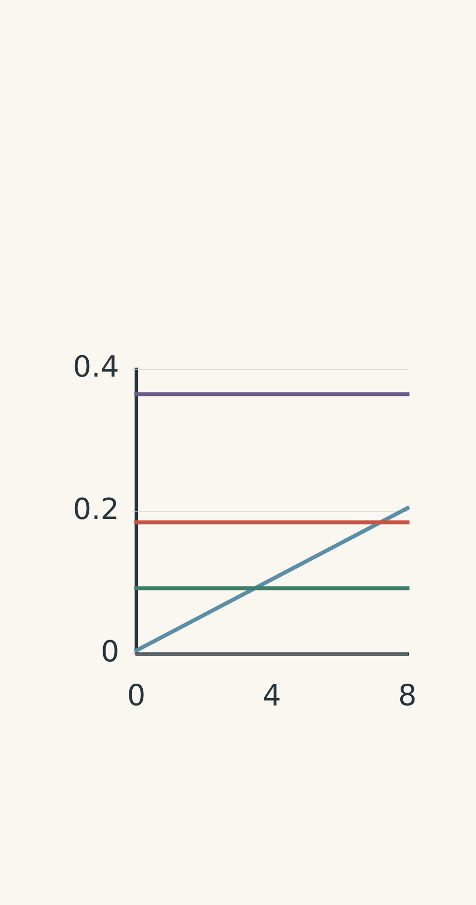
- Calibration line: 0–8.00 mg/L
- Dilution factor 10: A = 0.185
- Dilution factor 20: A = 0.0925
- Dilution factor 5: A = 0.365 (above range)
Solution 5
The best estimate of the original concentration is approximately \(71.0\ \mathrm{mg\,L^{-1}}\), using the first two measurements and excluding the third. The key is to judge the calibration range before deciding whether a calculated concentration is valid.
First, calculate the maximum absorbance covered by the standards:
\[
\begin{aligned}
A_{\max}
&=0.0250(8.00)+0.0050\\
&=0.205
\end{aligned}
\]
Any sample reading above 0.205 is outside the calibrated response range.
First aliquot: tenfold dilution
The diluted concentration is
\[
\begin{aligned}
c_1&=\frac{0.185-0.0050}
{0.0250\ \mathrm{L\,mg^{-1}}}\\
&=7.20\ \mathrm{mg\,L^{-1}}
\end{aligned}
\]
This concentration is within the calibrated range. The dilution factor is
\[
DF_1=\frac{10.00}{1.00}=10.0
\]
Therefore, the original concentration estimated from this aliquot is
\[
c_{\mathrm{original},1}
=7.20\times10.0
=72.0\ \mathrm{mg\,L^{-1}}
\]
Second aliquot: twentyfold dilution
The diluted concentration is
\[
\begin{aligned}
c_2&=\frac{0.0925-0.0050}
{0.0250\ \mathrm{L\,mg^{-1}}}\\
&=3.50\ \mathrm{mg\,L^{-1}}
\end{aligned}
\]
This result is also within the calibrated range. Its dilution factor is
\[
DF_2=\frac{20.00}{1.00}=20.0
\]
Therefore,
\[
c_{\mathrm{original},2}
=3.50\times20.0
=70.0\ \mathrm{mg\,L^{-1}}
\]
The two valid estimates are 72.0 mg/L and 70.0 mg/L. They are close, which supports their consistency under the assumptions given.
Because the question states that the two measurements have similar uncertainty, their mean is a reasonable estimate:
\[
\begin{aligned}
\bar{c}
&=\frac{72.0+70.0}{2}\\
&=71.0\ \mathrm{mg\,L^{-1}}
\end{aligned}
\]
Third aliquot: fivefold dilution
The absorbance of 0.365 is greater than the maximum calibrated response of 0.205. It is therefore outside the calibrated range.
The equation produces a mathematical concentration:
\[
\begin{aligned}
c_3&=\frac{0.365-0.0050}
{0.0250\ \mathrm{L\,mg^{-1}}}\\
&=14.4\ \mathrm{mg\,L^{-1}}
\end{aligned}
\]
Multiplying by the dilution factor of 5.00 gives 72.0 mg/L. That happens to agree with the first estimate, but it does not make the third measurement valid. The concentration of the solution actually measured, 14.4 mg/L, exceeds the highest standard concentration of 8.00 mg/L.
This is the central distinction: a plausible back-calculated result does not rescue a measurement taken outside the calibrated range.
Finally, the original concentration of approximately 71.0 mg/L is greater than 8.00 mg/L, but that is not a problem. The calibrated range applies to the diluted solutions entering the instrument, not necessarily to the original sample. Both measurements used in the estimate fall within the range supported by the standards.
10Next decision: is the concentration reliable?
Once you have calculated a concentration, the next step is to decide whether the measurement supports the conclusion you want to draw.
Check that the blank was handled consistently, the calibration relationship was appropriate, and the measured solution fell within the calibrated range. If you have replicate measurements, compare their back-calculated concentrations and investigate substantial differences rather than automatically averaging them.
For an HSC Chemistry response, make your reasoning visible: state the concentration and units, show the calibration calculation, apply every dilution factor, and explain why the result is supported by interpolation rather than extrapolation.
If the question asks whether a sample meets a concentration limit, compare the corrected original concentration with that limit. The calculation gives you a result; the calibration checks determine how confidently you can use it.