
Solenoid Induction Practical: Testing One Variable at a Time
Learn how to investigate the factors affecting induced emf in a solenoid using a fair-test method. Follow practical steps, apply Faraday’s law, analyse voltage readings, and work through HSC-style questions with detailed solutions.
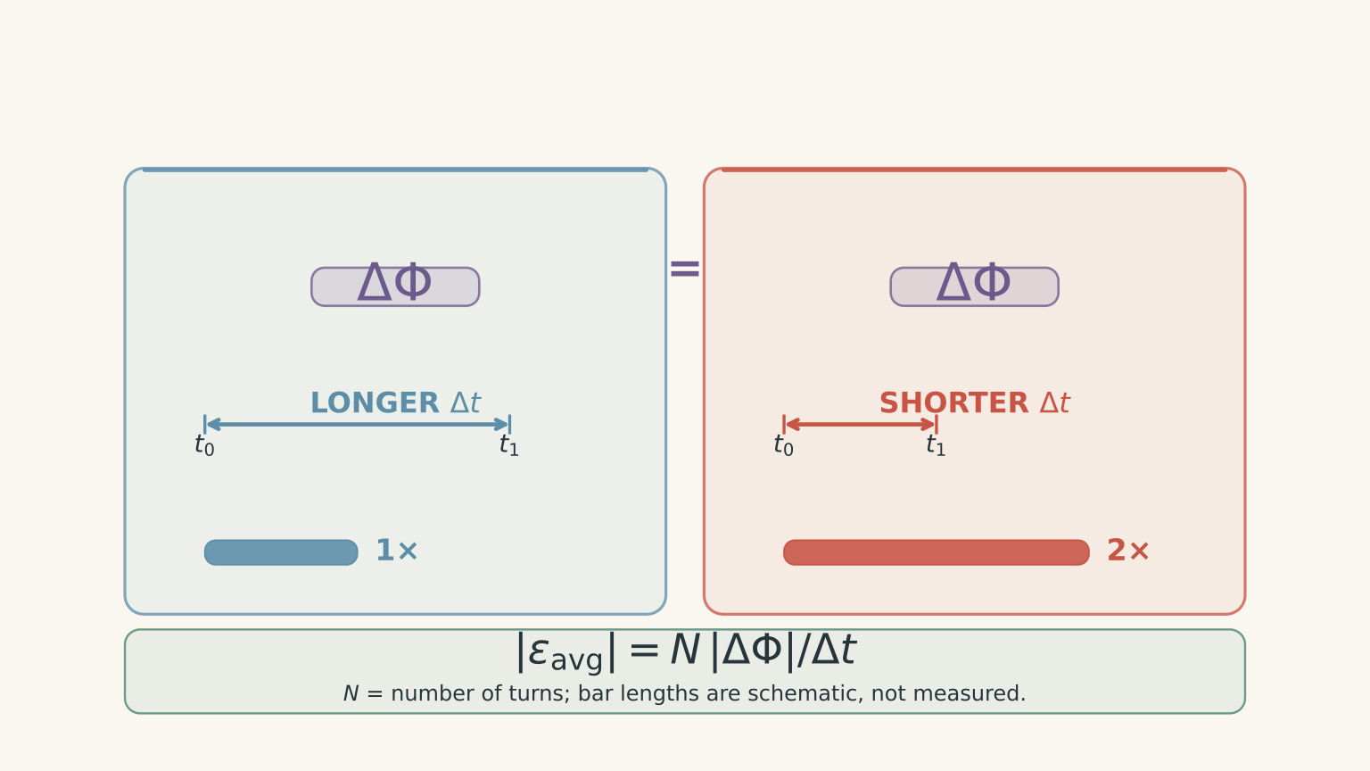
You slide the same bar magnet into the same solenoid twice. The second movement produces a taller voltage spike. Has the magnet caused a greater change in magnetic flux, or have you simply moved it faster?
Before reading on, predict what happens when the magnet travels between the same two positions in half the time.
If the change in magnetic flux per turn stays the same, the average induced emf doubles. The same change has happened in half the time. A taller voltage peak is consistent with this prediction, but the peak alone does not tell you everything about the flux change.
01The idea behind the practical
The purpose of this investigation is to test how different factors affect the induced electromotive force (emf) in a solenoid.
Magnetic flux measures how much magnetic field passes through the area enclosed by a coil turn. When the magnetic field through the turn changes, an emf is induced.
There are three factors worth investigating:
- How quickly the magnetic flux changes.
- How much the magnetic flux changes.
- How many turns the solenoid contains.
These factors are related, but they are not interchangeable.
Faraday’s law
Faraday’s law describes the relationship between induced emf and the change in magnetic flux linkage.
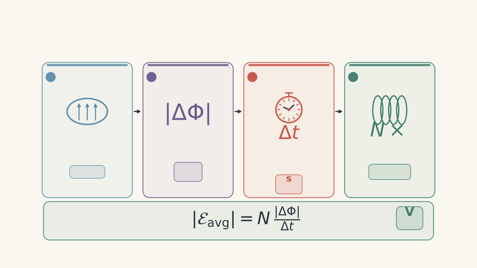
For a solenoid in which each turn experiences approximately the same magnetic flux, the average induced emf is
\[ \mathcal{E}_{\text{avg}}=-N\frac{\Delta\Phi}{\Delta t} \]
where:
- \(\mathcal{E}_{\text{avg}}\) is the average induced emf, measured in volts (V).
- \(N\) is the number of turns in the solenoid.
- \(\Delta\Phi\) is the change in magnetic flux through one turn, measured in webers (Wb).
- \(\Delta t\) is the time taken for that change, measured in seconds (s).
The negative sign represents Lenz’s law: the induced emf has a polarity that opposes the change producing it.
When comparing the sizes of induced emfs, we usually use the magnitude:
\[ |\mathcal{E}_{\text{avg}}| =N\frac{|\Delta\Phi|}{\Delta t} \]
This equation gives you three useful predictions.
| If you increase… | While keeping the other factors fixed | Expected result |
|---|---|---|
| The rate of flux change | Number of turns and total flux change | Greater average emf |
| The change in flux | Number of turns and time interval | Greater average emf |
| The number of turns | Flux change per turn and time interval | Greater average emf |
The first two rows are easy to confuse. A larger change in flux does not automatically produce a larger emf. You must also consider how long that change takes.
One way to picture this is to compare filling a bucket. Filling it with the same amount of water in two seconds rather than ten seconds means a greater flow rate. Here, the amount of water is like the change in flux, and the flow rate is like the rate of flux change. The analogy has a limit: magnetic flux is not a substance physically flowing through the coil.
Worked example: calculate the average induced emf
A solenoid has 500 turns. During one part of a magnet’s movement, the magnetic flux through each turn changes from \(0.10\ \text{mWb}\) to \(0.70\ \text{mWb}\) in \(0.040\ \text{s}\). Calculate the magnitude of the average induced emf.
Step 1
\[ \begin{aligned} |\Delta\Phi| &=0.70-0.10\\ &=0.60\ \text{mWb}\\ &=6.0\times10^{-4}\ \text{Wb} \end{aligned} \]
Remember that \(1\ \text{mWb}=10^{-3}\ \text{Wb}\).
Step 2
\[ \begin{aligned} |\mathcal{E}_{\text{avg}}| &=N\frac{|\Delta\Phi|}{\Delta t}\\ &=\frac{500(6.0\times10^{-4})}{0.040}\\ &=7.5\ \text{V} \end{aligned} \]
Step 3
The magnitude of the average induced emf is \(7.5\ \text{V}\). This is the average over the specified time interval, not necessarily the peak voltage displayed by a data logger.
That distinction will matter when you analyse your results.
02Design a fair test
A practical investigation needs three things:
- An independent variable: the factor you deliberately change.
- A dependent variable: the quantity you measure.
- Controlled variables: the conditions you keep constant.
The key rule is to change one independent variable at a time. If you change the magnet’s speed and the number of coil turns in the same comparison, you cannot tell which change caused the difference in emf.
Test 1: Does magnet speed affect induced emf?
Use the same magnet and solenoid. Move the magnet between the same starting and finishing positions, but take different amounts of time to complete the movement.
Keep constant:
- The solenoid and its number of turns.
- The magnet and its orientation.
- The starting and finishing positions.
- The path of the magnet.
- The voltage sensor and measurement interval.
Measure the time taken and the induced emf for each movement.
The change in flux per turn should be approximately the same because the magnet starts and finishes in the same positions relative to the same coil. The time taken is the factor you are deliberately changing.
Prediction: moving the magnet faster should increase the magnitude of the average induced emf.
For a fixed change in flux,
\[ |\mathcal{E}_{\text{avg}}|\propto\frac{1}{\Delta t} \]
The symbol \(\propto\) means “is proportional to”. Halving the time should double the average emf, provided the flux change remains the same.
Test 2: Does the number of turns affect induced emf?
Use matched solenoids with different numbers of turns. Keep their dimensions and magnetic environment as similar as possible.
Move the same magnet through the same path in the same time interval for each coil.
Keep constant:
- The magnet and its orientation.
- The starting and finishing positions.
- The time taken for the movement.
- The coil’s diameter, length, and core, as far as the available equipment allows.
- The measurement method.
Change only the number of turns, \(N\).
Prediction: increasing the number of turns should increase the induced emf, provided the change in flux per turn and the time interval remain the same.
For example, doubling the number of turns should double the average induced emf under these conditions.
One experimental detail matters here. Coils with more turns can have different wire lengths and resistances. A high-input-impedance voltage sensor minimises the effect of these differences on the measured voltage by drawing very little current.
Test 3: Does the size of the flux change affect induced emf?
This investigation needs a little more care.
One practical approach is to use the same solenoid and magnet, keep the starting position fixed, and vary the finishing position. Complete each movement in the same time interval.
A different finishing position generally produces a different final magnetic flux through the coil. This changes the total flux change during the movement.
Keep constant:
- The solenoid and number of turns.
- The magnet and its orientation.
- The starting position.
- The duration of the movement.
- The voltage sensor and the measurement interval.
Change only the finishing position.
Prediction: a larger change in magnetic flux should produce a larger average induced emf if the time interval and number of turns are fixed.
There is an important limitation. The magnet’s finishing position is a practical way to change the flux, but it is not a direct measurement of \(\Delta\Phi\). Unless you measure or independently determine the flux change, describe position as a proxy for flux change rather than claiming you have measured flux directly.
Also, use the average emf for this comparison. Changing the finishing position can change the magnet’s speed profile, so comparing peak voltages alone may introduce another source of variation.
Three fair tests: change one variable at a time
| 01 · SPEED TEST | CHANGE: Transit time CONTROL: Same coil, magnet and starting and finishing positions MEASURE: Average induced emf |
|---|---|
| 02 · TURNS TEST | CHANGE: Number of turns, N CONTROL: Same magnet movement and coil geometry as far as possible MEASURE: Average induced emf |
| 03 · FLUX-CHANGE TEST | CHANGE: Magnet’s finishing position (a proxy for ΔΦ) CONTROL: Same N, starting position and total movement time MEASURE: Average induced emf NOTE: Finishing position changes the flux indirectly; it does not directly measure ΔΦ. |
03Run the practical
You do not need to investigate all three factors in one experimental series. In fact, separating the tests makes your conclusions much stronger.
Equipment
You will need:
- A solenoid, or a set of matched solenoids with different numbers of turns.
- A bar magnet.
- A high-input-impedance voltage sensor and data logger, if available.
- A ruler or another way to mark repeatable starting and finishing positions.
- A timer, motion sensor, or slow-motion video to estimate movement time.
- A computer or notebook for recording results.
A data logger is particularly useful because the induced emf may be a short-lived pulse. A standard multimeter can miss the peak or fail to display the transient clearly.
Step 1: Set up your measurement
Connect the voltage sensor across the solenoid and check that the sensor is zeroed and set to a suitable voltage range.
Use the same sensor settings throughout a comparison. If the voltage exceeds the selected range, the signal may be clipped, making the recorded peak artificially low.
Choose one part of the movement to analyse, such as the magnet’s approach from a marked starting position to a marked finishing position.
Do not automatically analyse the entire journey into and out of the coil as one interval. The induced emf can reverse polarity between the approach and departure phases. If you average the signed voltage across the complete movement, the positive and negative parts may cancel, even though substantial induction occurred.
Step 2: Collect a baseline reading
Complete the chosen movement several times using the same conditions.
Record the measured emf, the movement time, and any obvious inconsistencies. This gives you a baseline against which to compare later trials.
If the results vary substantially, check whether the magnet followed the same path, whether the timing was accurate, and whether the sensor captured the full voltage pulse.
Step 3: Change one factor
Run each investigation as a separate series.
For the speed test, use the same starting and finishing positions but different movement times.
For the turns test, change the solenoid while keeping the magnet’s movement as consistent as possible.
For the flux-change test, use the same starting position and duration but vary the finishing position.
If the movement is too fast to time reliably with a handheld stopwatch, use slow-motion video or a motion sensor if available. Human reaction time can be a substantial fraction of a short movement interval.
Step 4: Repeat each condition
Aim for at least three trials at each setting.
Calculate the mean of repeated readings taken under the same conditions. Repeats help reveal random variation, but they do not correct a systematic error, such as using different coil geometries or measuring only part of the voltage pulse.
Keep the signed readings if you are investigating polarity. When comparing emf magnitudes, compare readings consistently and state that you are using their magnitudes.
Step 5: Record your results
A useful results table separates the manipulated variable from the measured response.
| Run | Factor tested and setting | \(N\) | \(\Delta t\) (s) | Mean emf magnitude (V) | Peak emf magnitude (V) |
|---|---|---|---|---|---|
| 1 | |||||
| 2 | |||||
| 3 |
Record the starting and finishing positions in your notes, too. They are especially important when you are trying to keep the flux change constant.
Do not mix peak emf and average emf in the same comparison without clearly distinguishing them. They are different measurements and need not change by exactly the same ratio.
04Interpret the results
Once you have collected the data, use Faraday’s law to decide whether the results support your prediction.
Look for the expected relationship
| Investigation | Expected relationship | Useful graph |
|---|---|---|
| Magnet speed | Average emf increases as the time interval decreases, for the same flux change and number of turns. | Mean emf against \(1/\Delta t\). |
| Number of turns | Average emf is proportional to \(N\), if flux change per turn and time are fixed. | Mean emf against number of turns. |
| Flux change | Average emf is proportional to \(|\Delta\Phi|\), if \(N\) and time are fixed. | Mean emf against measured flux change, if available. |
For the speed test, plotting mean emf against \(1/\Delta t\) is useful because Faraday’s law predicts a linear relationship when the flux change and number of turns are constant.
For the turns test, a graph of mean emf against \(N\) should also be approximately linear under controlled conditions.
For the flux-change test, a graph against finishing position may show a trend, but it need not be a straight line. Magnetic flux does not necessarily change linearly with the magnet’s position.
Example: interpreting speed-test data
Suppose an illustrative experiment uses the same coil and the same starting and finishing positions for every trial. The measured results are:
| Time interval, \(\Delta t\) (s) | \(1/\Delta t\) (s\(^{-1}\)) | Mean emf magnitude (V) |
|---|---|---|
| 0.40 | 2.50 | 0.48 |
| 0.25 | 4.00 | 0.79 |
| 0.16 | 6.25 | 1.20 |
These are illustrative values, not measurements from a real experiment.
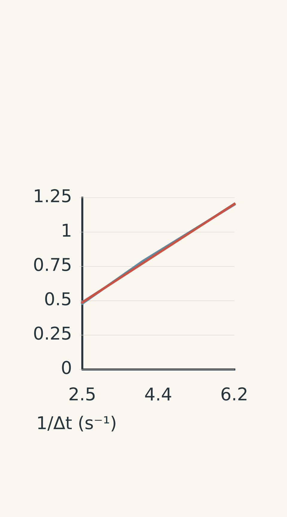
- Illustrative measurements
- Approximate linear best-fit trend
The graph shows that the mean emf increases as the time interval decreases.
You can also check whether the product of emf and time remains approximately constant:
\[ |\mathcal{E}_{\text{avg}}|\Delta t \]
For the three trials, the products are approximately \(0.192\), \(0.198\), and \(0.192\ \text{V\,s}\).
These values are close. Since
\[ |\mathcal{E}_{\text{avg}}|\Delta t=N|\Delta\Phi| \]
the results support the prediction that the flux change was approximately constant while the rate of change varied.
The small differences are plausible experimental variation. They could arise from timing uncertainty, slight differences in the magnet’s path, or limitations in the voltage sensor.
What can weaken your conclusion?
A practical result is only as convincing as the controls behind it.
- Inconsistent movement: If the magnet follows a different path or starts from a different position, the flux change may not be constant.
- Poor timing: Short movements are difficult to time accurately by hand. Use video or a motion sensor where possible.
- Different coil geometry: Changing the number of turns can also change the coil’s dimensions or its coupling to the magnet.
- Missed voltage peaks: A sensor that samples too slowly may underestimate the peak emf.
- Changing more than one factor: If speed, coil turns, and magnet position all change together, the cause of the result is unclear.
- Averaging the wrong interval: Including both entry and exit can cause opposite-polarity signals to cancel.
If you have only one lesson to complete the investigation, the speed test is a sensible starting point. It needs only one coil and one magnet, and the starting and finishing positions can be controlled. If your equipment includes matched coils and a reliable voltage sensor, you can then investigate the effect of turns. The flux-change test is also useful, but it requires careful interpretation of the finishing position and the measured time interval.
05Questions and solutions
Question 1
A solenoid has 250 turns. During one part of a magnet’s movement, the magnetic flux through each turn changes from \(0.10\ \text{mWb}\) to \(0.70\ \text{mWb}\) in \(0.075\ \text{s}\).
Calculate the magnitude of the average induced emf.
Solution 1
The magnitude of the average induced emf is \(2.0\ \text{V}\).
First, calculate the change in flux per turn:
\[ \begin{aligned} |\Delta\Phi| &=0.70-0.10\\ &=0.60\ \text{mWb}\\ &=6.0\times10^{-4}\ \text{Wb} \end{aligned} \]
Apply Faraday’s law:
\[ \begin{aligned} |\mathcal{E}_{\text{avg}}| &=N\frac{|\Delta\Phi|}{\Delta t}\\ &=\frac{250(6.0\times10^{-4})}{0.075}\\ &=2.0\ \text{V} \end{aligned} \]
The answer is the average emf over the specified interval. It is not necessarily the maximum voltage recorded during the movement.
Question 2
A student investigates magnet speed using a 400-turn solenoid. The same magnet is moved between the same starting and finishing positions in each trial.
The results are:
| Trial | Time interval (s) | Mean emf magnitude (V) |
|---|---|---|
| Slow | 0.30 | 0.80 |
| Fast | 0.12 | 1.95 |
(a) Are the results consistent with Faraday’s law? Justify your answer quantitatively.
(b) Estimate the change in magnetic flux per turn for each trial.
(c) Identify two experimental checks that would help explain any difference between the inferred flux changes.
Solution 2
The results are approximately consistent with Faraday’s law: the faster movement produces a larger mean emf, and the inferred flux changes are very similar.
(a) If the flux change and number of turns are constant, Faraday’s law predicts
\[ |\mathcal{E}_{\text{avg}}|\propto\frac{1}{\Delta t} \]
The expected ratio of fast to slow emf is
\[ \frac{|\mathcal{E}_{\text{fast}}|} {|\mathcal{E}_{\text{slow}}|} =\frac{0.30}{0.12} =2.50 \]
The measured ratio is
\[ \frac{1.95}{0.80}=2.44 \]
The measured ratio is close to the predicted value of \(2.50\).
(b) Rearrange Faraday’s law to calculate the magnitude of the flux change per turn:
\[ |\Delta\Phi| =\frac{|\mathcal{E}_{\text{avg}}|\Delta t}{N} \]
For the slow trial:
\[ \begin{aligned} |\Delta\Phi_{\text{slow}}| &=\frac{0.80(0.30)}{400}\\ &=6.0\times10^{-4}\ \text{Wb}\\ &=0.600\ \text{mWb} \end{aligned} \]
For the fast trial:
\[ \begin{aligned} |\Delta\Phi_{\text{fast}}| &=\frac{1.95(0.12)}{400}\\ &=5.85\times10^{-4}\ \text{Wb}\\ &=0.585\ \text{mWb} \end{aligned} \]
The difference is small: \(0.015\ \text{mWb}\), or approximately \(2.5\%\) of the slow-trial estimate.
(c) Two useful checks are:
- Confirm that the magnet started and finished at exactly the same positions, with the same orientation, in both trials.
- Repeat the measurements and check that the sensor captured the entire voltage pulse and that the timing method was reliable.
The small discrepancy does not automatically disprove Faraday’s law. It may reflect ordinary experimental uncertainty.
Question 3
A student uses three matched solenoids to investigate the effect of the number of turns. The magnet follows the same path in the same time for every trial.
The measured mean emf magnitudes are:
| Number of turns, \(N\) | Mean emf magnitude (V) |
|---|---|
| 200 | 0.72 |
| 400 | 1.49 |
| 600 | 2.18 |
(a) Explain whether the results support the prediction that induced emf is proportional to the number of turns.
(b) Estimate the mean emf magnitude for an 800-turn solenoid under the same conditions.
(c) Give one reason the measured values might not be exactly proportional to the number of turns.
Solution 3
The results support an approximately proportional relationship, and an 800-turn solenoid would be expected to produce a mean emf of about \(2.9\ \text{V}\).
(a) Faraday’s law gives
\[ |\mathcal{E}_{\text{avg}}| =N\frac{|\Delta\Phi|}{\Delta t} \]
If the flux change per turn and the time interval remain constant, the mean emf should be proportional to \(N\).
Check the emf per turn:
\[ \begin{aligned} \frac{0.72}{200} &=0.00360\ \text{V per turn}\\ \frac{1.49}{400} &=0.003725\ \text{V per turn}\\ \frac{2.18}{600} &\approx0.00363\ \text{V per turn} \end{aligned} \]
These values are similar. The mean emf approximately doubles when the number of turns doubles, and approximately triples when the number of turns triples.
(b) Using the 200-turn result as a proportional estimate:
\[ \begin{aligned} |\mathcal{E}_{800}| &\approx0.72\left(\frac{800}{200}\right)\\ &=2.88\ \text{V} \end{aligned} \]
A reasonable prediction is approximately \(2.9\ \text{V}\).
(c) The coils may not have exactly the same dimensions or magnetic coupling. A different coil diameter or length could change the flux through each turn, meaning that the assumption of a constant flux change per turn is no longer perfectly satisfied.
The important point is that proportionality depends on the controlled conditions, not just on the number of turns.
Question 4
A 500-turn solenoid is used in two trials. The change in magnetic flux per turn and the time interval are:
| Trial | Flux change per turn (mWb) | Time interval (s) |
|---|---|---|
| A | 0.30 | 0.10 |
| B | 0.75 | 0.25 |
(a) Calculate the magnitude of the average induced emf in each trial.
(b) A student argues that trial B must produce a larger emf because the flux change is greater. Explain why this prediction is incorrect.
(c) Describe how you would design a practical investigation to test the effect of flux change more fairly.
Solution 4
Both trials produce an average induced emf of \(1.5\ \text{V}\). Trial B has a greater flux change, but that change also takes proportionally longer.
(a) For trial A:
\[ \begin{aligned} |\mathcal{E}_{A}| &=\frac{500(0.30\times10^{-3})}{0.10}\\ &=1.5\ \text{V} \end{aligned} \]
For trial B:
\[ \begin{aligned} |\mathcal{E}_{B}| &=\frac{500(0.75\times10^{-3})}{0.25}\\ &=1.5\ \text{V} \end{aligned} \]
The average emf magnitudes are equal.
(b) Trial B has \(2.5\) times the flux change of trial A:
\[ \frac{0.75}{0.30}=2.5 \]
However, it also takes \(2.5\) times as long:
\[ \frac{0.25}{0.10}=2.5 \]
The increase in flux change is exactly balanced by the increase in time. The average rate of change of flux per turn is therefore the same in both trials.
The tempting mistake is to consider only \(\Delta\Phi\) and ignore \(\Delta t\). Faraday’s law depends on their ratio.
(c) Use the same solenoid and magnet, keep the starting position fixed, and vary only the finishing position. Complete each movement in the same time interval and measure the mean induced emf over the same type of movement.
This changes the flux change while holding the number of turns and time interval constant. If the finishing position is used as a proxy for flux change, state that limitation clearly. Use the mean emf rather than relying only on peak voltage, because the movement profile may differ between trials.
Question 5
Two matched solenoids are used to investigate the effect of the number of turns. Solenoid A has 200 turns, and solenoid B has 400 turns. Their dimensions and magnetic environments are otherwise matched.
The same magnet moves between the same starting and finishing positions during one monotonic entry phase in each trial. However, the movement takes different amounts of time.
A voltage data logger records the following approximately triangular, positive emf pulses:
- Solenoid A: peak emf \(4.0\ \text{V}\), pulse duration \(0.10\ \text{s}\).
- Solenoid B: peak emf \(4.0\ \text{V}\), pulse duration \(0.20\ \text{s}\).
Assume each pulse represents the entire entry phase and that the triangular approximation is suitable for estimating the area under each voltage-time graph.
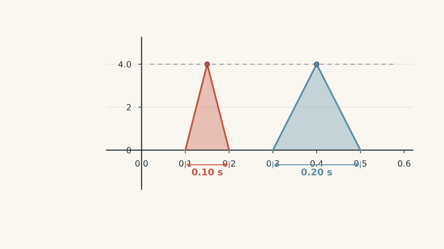
A student concludes that doubling the number of turns has no effect on induced emf because the peak readings are identical.
(a) Calculate the area under each voltage-time pulse.
(b) Use these areas to calculate the magnitude of the change in magnetic flux per turn for each solenoid.
(c) Calculate the average emf for each pulse and assess the student’s conclusion.
(d) Explain how the student could redesign the comparison to test the effect of the number of turns fairly.
Solution 5
The student’s conclusion is not justified. The two peak readings are identical because the increased number of turns in solenoid B is accompanied by a longer movement time. The data are consistent with the same flux change per turn occurring over twice the time.
(a) For an approximately triangular pulse, the area is
\[ \text{Area}=\frac{1}{2} \times\text{base}\times\text{height} \]
For solenoid A:
\[ \begin{aligned} \text{Area}_A &=\frac{1}{2}(0.10)(4.0)\\ &=0.20\ \text{V\,s} \end{aligned} \]
For solenoid B:
\[ \begin{aligned} \text{Area}_B &=\frac{1}{2}(0.20)(4.0)\\ &=0.40\ \text{V\,s} \end{aligned} \]
The area under a single-polarity emf-time pulse represents the magnitude of the change in flux linkage. Since \(1\ \text{V\,s}=1\ \text{Wb}\), the areas can be used to infer the flux change per turn.
(b) For solenoid A, the magnitude of the flux change per turn is
\[ \begin{aligned} |\Delta\Phi_A| &=\frac{\text{Area}_A}{N_A}\\ &=\frac{0.20}{200}\\ &=0.0010\ \text{Wb}\\ &=1.0\ \text{mWb} \end{aligned} \]
For solenoid B:
\[ \begin{aligned} |\Delta\Phi_B| &=\frac{\text{Area}_B}{N_B}\\ &=\frac{0.40}{400}\\ &=0.0010\ \text{Wb}\\ &=1.0\ \text{mWb} \end{aligned} \]
Both solenoids experience the same change in magnetic flux per turn, as expected from the matched geometry and identical starting and finishing positions.
Notice that doubling the number of turns doubles the area under the voltage-time pulse. The peak alone does not reveal this difference.
(c) The average emf is the area under the pulse divided by its duration.
For solenoid A:
\[ |\mathcal{E}_{A,\text{avg}}| =\frac{0.20}{0.10} =2.0\ \text{V} \]
For solenoid B:
\[ |\mathcal{E}_{B,\text{avg}}| =\frac{0.40}{0.20} =2.0\ \text{V} \]
Both average emf magnitudes are \(2.0\ \text{V}\), and both peak readings are \(4.0\ \text{V}\).
There is no contradiction with Faraday’s law. Solenoid B has twice as many turns, but the flux change takes twice as long. Its average rate of flux change per turn is therefore half that of solenoid A. Doubling \(N\) while halving the rate of flux change leaves the product unchanged.
The student has changed two factors together: the number of turns and the movement time. The identical peak readings cannot establish that the number of turns has no effect.
(d) The student should repeat the comparison using the same magnet, starting and finishing positions, movement time, and orientation for both solenoids. The coil dimensions and magnetic environment should be matched as closely as possible, and the same high-input-impedance voltage sensor should be used.
The average emf should then be compared over the same movement interval. If the flux change per turn is the same and the movement time is controlled, doubling the number of turns should double the average induced emf.
This investigation also leads naturally to Lenz’s law. Once you can control and explain the magnitude of the induced emf, you can reverse the magnet’s orientation or the direction of movement and investigate how the polarity changes. The same experimental discipline still applies: change one factor at a time, control the others, and make sure your measurements answer the question you intended to test.