
Calculate Solubility from Ksp for HSC Chemistry
Learn how to calculate molar solubility from Ksp using balanced dissolution equations, ion ratios, and equilibrium concentrations. Includes worked examples and challenging HSC-style questions.
A question gives you \(K_{sp}=3.9\times10^{-11}\) for calcium fluoride and asks for its solubility. The tempting move is to write \(3.9\times10^{-11}\ \mathrm{mol\,L^{-1}}\) and move on.
Predict before reading further: is that actually the solubility?
No. \(K_{sp}\) is built from the equilibrium concentrations of the ions, not directly from the amount of solid that dissolves. For calcium fluoride, every mole of solid that dissolves produces one mole of calcium ions and two moles of fluoride ions. That \(1:2\) ratio changes the calculation completely.
The key skill is translating a balanced dissolution equation into ion concentrations.
01From one dissolved formula unit to ion concentrations
Start with calcium fluoride:
\[ \ce{CaF2(s) <=> Ca^2+(aq) + 2F^-(aq)} \]
Suppose its molar solubility is \(s\ \mathrm{mol\,L^{-1}}\). That means \(s\) moles of \(\ce{CaF2}\) dissolve per litre of saturated solution.
The balanced equation then tells us:
\[ [\mathrm{Ca}^{2+}]=s \]
and
\[ [\mathrm{F}^{-}]=2s \]
Think of each formula unit of \(\ce{CaF2}\) as one student arriving with two friends. If \(s\) groups arrive, you get \(s\) calcium ions and \(2s\) fluoride ions.
The analogy stops there. Once dissolved, the ions are not wandering around in little groups of three. The balanced equation only tells us the ratio in which they are produced.
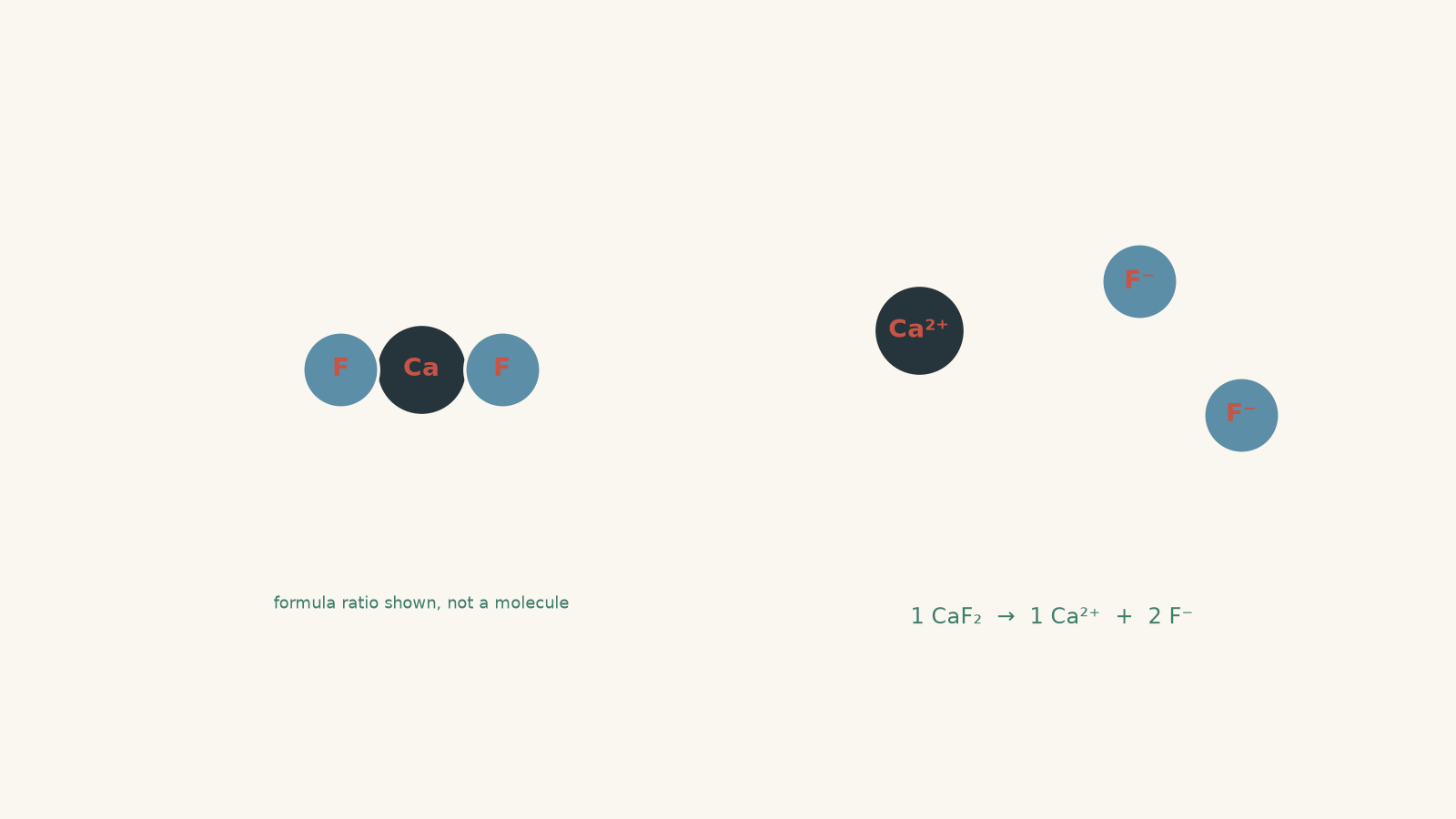
This first model assumes the water did not already contain calcium or fluoride ions. We will remove that assumption later.
02What \(K_{sp}\) actually measures
For a sparingly soluble ionic solid, dissolution eventually reaches a dynamic equilibrium. Ions continue leaving and joining the solid, but their equilibrium concentrations stay constant.
For calcium fluoride,
\[ \ce{CaF2(s) <=> Ca^2+(aq) + 2F^-(aq)} \]
the solubility product expression is
\[ K_{sp}=[\mathrm{Ca}^{2+}][\mathrm{F}^{-}]^2 \]
The solid \(\ce{CaF2}\) does not appear in the expression. A pure solid has effectively constant activity while it is present, so its amount is not included as a concentration term.
Now substitute the concentrations created by dissolving \(s\ \mathrm{mol\,L^{-1}}\):
\[ K_{sp}=s(2s)^2=4s^3 \]
So
\[ s=\sqrt[3]{\frac{K_{sp}}{4}} \]
That is why \(K_{sp}\) itself is not the solubility.
The coefficients do two different jobs
This is one of the easiest places to lose marks.
In
\[ \ce{CaF2(s) <=> Ca^2+(aq) + 2F^-(aq)} \]
the coefficient \(2\) tells you that
\[ [\mathrm{F}^{-}]=2s \]
but it also becomes an exponent in the \(K_{sp}\) expression:
\[ K_{sp}=[\mathrm{Ca}^{2+}][\mathrm{F}^{-}]^2 \]
So the calculation contains both pieces:
\[ K_{sp}=s(2s)^2 \]
Using \(s^3\), or using \(s(2s)\), misses part of the chemistry.
03A reliable method for converting \(K_{sp}\) into solubility
For a saturated solution in pure water, with no important side reactions:
- Write the balanced dissolution equation.
- Let the molar solubility equal \(s\).
- Use the coefficients to write each equilibrium ion concentration in terms of \(s\).
- Write the \(K_{sp}\) expression.
- Substitute the ion concentrations.
- Solve for \(s\).
- Convert to another unit, such as \(\mathrm{g\,L^{-1}}\), only if asked.
Some common patterns are worth recognising.
| Dissolution pattern | Concentrations produced by solubility \(s\) | \(K_{sp}\) relationship |
|---|---|---|
| \(\ce{MX(s) <=> M(aq) + X(aq)}\) | \(s,\ s\) | \(K_{sp}=s^2\) |
| \(\ce{MX2(s) <=> M(aq) + 2X(aq)}\) | \(s,\ 2s\) | \(K_{sp}=4s^3\) |
| \(\ce{M2X(s) <=> 2M(aq) + X(aq)}\) | \(2s,\ s\) | \(K_{sp}=4s^3\) |
| \(\ce{M2X3(s) <=> 2M(aq) + 3X(aq)}\) | \(2s,\ 3s\) | \(K_{sp}=108s^5\) |
Do not memorise this table instead of using the equation. The balanced equation is safer because unfamiliar stoichiometries can always be rebuilt from first principles.
Worked example: solubility of a 1:1 salt
A saturated solution of \(\ce{AgCl}\) has \(K_{sp}=1.8\times10^{-10}\) at the stated temperature. Calculate its molar solubility and its solubility in \(\mathrm{g\,L^{-1}}\). The molar mass of \(\ce{AgCl}\) is \(143.3\ \mathrm{g\,mol^{-1}}\).
Step 1
\[ \ce{AgCl(s) <=> Ag+(aq) + Cl-(aq)} \]
Step 2
One mole of \(\ce{AgCl}\) produces one mole of each ion, so
\[ [\mathrm{Ag}^{+}]=s,\qquad [\mathrm{Cl}^{-}]=s \]
Step 3
\[ K_{sp}=[\mathrm{Ag}^{+}][\mathrm{Cl}^{-}]=s^2 \]
Therefore,
\[ 1.8\times10^{-10}=s^2 \]
Step 4
\[ s=\sqrt{1.8\times10^{-10}} =1.34\times10^{-5}\ \mathrm{mol\,L^{-1}} \]
Step 5
\[ \begin{aligned} \text{mass solubility} &=(1.34\times10^{-5})(143.3)\\ &=1.92\times10^{-3}\ \mathrm{g\,L^{-1}} \end{aligned} \]
So only about \(1.92\ \mathrm{mg}\) of \(\ce{AgCl}\) dissolves per litre under these conditions.
The important feature here is the \(1:1\) dissolution ratio. Even for this simplest case, \(K_{sp}\neq s\); instead, \(K_{sp}=s^2\).
Worked example: when one ion is produced twice
Assume \(\ce{CaF2}\) has \(K_{sp}=3.9\times10^{-11}\) at the stated temperature. Calculate its molar solubility in pure water and its mass solubility. The molar mass of \(\ce{CaF2}\) is \(78.07\ \mathrm{g\,mol^{-1}}\). Ignore other equilibria.
Step 1
\[ \ce{CaF2(s) <=> Ca^2+(aq) + 2F^-(aq)} \]
Step 2
\[ [\mathrm{Ca}^{2+}]=s,\qquad [\mathrm{F}^{-}]=2s \]
Step 3
\[ K_{sp}=[\mathrm{Ca}^{2+}][\mathrm{F}^{-}]^2 \]
Substituting gives
\[ 3.9\times10^{-11}=s(2s)^2=4s^3 \]
Step 4
\[ \begin{aligned} s^3&=\frac{3.9\times10^{-11}}{4}\\ &=9.75\times10^{-12} \end{aligned} \]
Therefore,
\[ s=2.14\times10^{-4}\ \mathrm{mol\,L^{-1}} \]
Notice that the solubility is millions of times larger than the numerical value of \(K_{sp}\). They are different quantities connected by the dissolution stoichiometry.
Step 5
\[ \begin{aligned} \text{mass solubility} &=(2.14\times10^{-4})(78.07)\\ &=1.67\times10^{-2}\ \mathrm{g\,L^{-1}} \end{aligned} \]
So the solution contains about \(0.0167\ \mathrm{g}\) of dissolved \(\ce{CaF2}\) per litre at saturation.
04The most tempting wrong shortcut
A smaller \(K_{sp}\) often suggests a sparingly soluble substance, but you cannot safely compare the solubilities of two salts just by comparing their \(K_{sp}\) values.
Suppose Salt A dissolves \(1:1\):
\[ \ce{MX(s) <=> M(aq) + X(aq)} \]
Then
\[ K_{sp}=s^2 \]
But Salt B dissolves \(1:2\):
\[ \ce{MY2(s) <=> M(aq) + 2Y(aq)} \]
and therefore
\[ K_{sp}=4s^3 \]
The same molar solubility produces completely different \(K_{sp}\) values because the equilibrium expressions have different powers.
So the decision rule is simple: compare molar solubilities only after converting each \(K_{sp}\) through its own balanced dissolution equation.
A few other traps are worth watching.
| Tempting move | Why it fails |
|---|---|
| Set \(s=K_{sp}\) | \(K_{sp}\) is a product of equilibrium ion concentrations. |
| Give every ion concentration as \(s\) | Coefficients in the dissolution equation may produce \(2s\), \(3s\), and so on. |
| Use coefficients only as exponents | The coefficients also determine the ion concentrations before you substitute. |
| Include the solid in the \(K_{sp}\) expression | Pure solids are omitted from the equilibrium expression. |
| Rank different salts by \(K_{sp}\) alone | Different dissolution stoichiometries give different mathematical relationships between \(K_{sp}\) and \(s\). |
05When \([\text{ion}]=\text{coefficient}\times s\) stops being enough
So far, every calculation has started with pure water.
Now imagine dissolving \(\ce{CaF2}\) in a solution that already contains \(0.0100\ \mathrm{mol\,L^{-1}}\) fluoride ions from soluble \(\ce{NaF}\).
If another \(s\ \mathrm{mol\,L^{-1}}\) of \(\ce{CaF2}\) dissolves,
\[ [\mathrm{Ca}^{2+}]=s \]
but the fluoride concentration is not \(2s\). It is
\[ [\mathrm{F}^{-}]=0.0100+2s \]
Therefore,
\[ K_{sp}=s(0.0100+2s)^2 \]
The balanced equation has not changed. What changed is the starting concentration.
This is the common-ion effect: adding an ion already present in the dissolution equilibrium usually reduces the amount of solid that can dissolve.
There is one more distinction that becomes important when solutions are mixed. \(K_{sp}\) describes the saturated equilibrium. The ion product,
\[ Q_{sp} \]
uses the same expression but the concentrations that exist right now.
- If \(Q_{sp}K_{sp}\), precipitation is favoured until the ion concentrations fall.
If deciding whether a precipitate forms is still shaky, revise Solubility Rules and Precipitation Tests for HSC Chemistry.
06Questions and solutions
Question 1
At a particular temperature, \(\ce{PbSO4}\) has \(K_{sp}=1.6\times10^{-8}\).
\[ \ce{PbSO4(s) <=> Pb^2+(aq) + SO4^2-(aq)} \]
Calculate its molar solubility in pure water. Assume no other equilibria are significant.
Solution 1
The molar solubility is \(1.3\times10^{-4}\ \mathrm{mol\,L^{-1}}\).
Let the molar solubility be \(s\). The dissolution equation is \(1:1\), so
\[ [\mathrm{Pb}^{2+}]=s,\qquad [\ce{SO4^2-}]=s \]
The solubility product expression is
\[ K_{sp}=[\mathrm{Pb}^{2+}][\ce{SO4^2-}] \]
Therefore,
\[ \begin{aligned} 1.6\times10^{-8}&=s^2\\ s&=\sqrt{1.6\times10^{-8}}\\ &=1.26\times10^{-4}\ \mathrm{mol\,L^{-1}} \end{aligned} \]
To two significant figures,
\[ s=1.3\times10^{-4}\ \mathrm{mol\,L^{-1}} \]
The tempting mistake is to report \(1.6\times10^{-8}\ \mathrm{mol\,L^{-1}}\). That number is \(K_{sp}\), not the concentration of dissolved \(\ce{PbSO4}\).
Question 2
Silver chromate dissolves according to
\[ \ce{Ag2CrO4(s) <=> 2Ag+(aq) + CrO4^2-(aq)} \]
At a particular temperature, \(K_{sp}=1.10\times10^{-12}\).
Calculate:
- the molar solubility of \(\ce{Ag2CrO4}\) in pure water,
- the equilibrium concentration of \(\mathrm{Ag}^{+}\), and
- the mass of \(\ce{Ag2CrO4}\) dissolved in \(250.0\ \mathrm{mL}\) of saturated solution.
Use a molar mass of \(331.7\ \mathrm{g\,mol^{-1}}\).
Solution 2
The molar solubility is \(6.50\times10^{-5}\ \mathrm{mol\,L^{-1}}\), the silver ion concentration is \(1.30\times10^{-4}\ \mathrm{mol\,L^{-1}}\), and \(5.39\times10^{-3}\ \mathrm{g}\) of \(\ce{Ag2CrO4}\) is dissolved in \(250.0\ \mathrm{mL}\).
Let the molar solubility be \(s\).
From
\[ \ce{Ag2CrO4(s) <=> 2Ag+(aq) + CrO4^2-(aq)} \]
we have
\[ [\mathrm{Ag}^{+}]=2s,\qquad [\ce{CrO4^2-}]=s \]
The equilibrium expression is
\[ K_{sp}=[\mathrm{Ag}^{+}]^2[\ce{CrO4^2-}] \]
so
\[ \begin{aligned} 1.10\times10^{-12} &=(2s)^2(s)\\ &=4s^3 \end{aligned} \]
Hence
\[ \begin{aligned} s&=\sqrt[3]{\frac{1.10\times10^{-12}}{4}}\\ &=6.50\times10^{-5}\ \mathrm{mol\,L^{-1}} \end{aligned} \]
The silver ion concentration is twice this:
\[ [\mathrm{Ag}^{+}] =2(6.50\times10^{-5}) =1.30\times10^{-4}\ \mathrm{mol\,L^{-1}} \]
Now calculate how many moles of solid are dissolved in \(0.2500\ \mathrm{L}\):
\[ \begin{aligned} n&=cV\\ &=(6.50\times10^{-5})(0.2500)\\ &=1.63\times10^{-5}\ \mathrm{mol} \end{aligned} \]
Therefore,
\[ \begin{aligned} m&=nM\\ &=(1.63\times10^{-5})(331.7)\\ &=5.39\times10^{-3}\ \mathrm{g} \end{aligned} \]
The trap is using \(s\) for both ion concentrations. There are twice as many dissolved silver ions as dissolved chromate ions.
Question 3
Two hypothetical salts are examined at the same temperature.
Salt A dissolves according to
\[ \ce{MX(s) <=> M^2+(aq) + X^2-(aq)} \]
and has
\[ K_{sp}=1.0\times10^{-8} \]
Salt B dissolves according to
\[ \ce{MY2(s) <=> M^2+(aq) + 2Y^-(aq)} \]
and has
\[ K_{sp}=3.2\times10^{-11} \]
A student claims Salt A must have the greater molar solubility because its \(K_{sp}\) is more than 300 times larger.
Determine which salt actually has the greater molar solubility, and calculate the total concentration of dissolved ions produced by each saturated solution.
Solution 3
Salt B has the greater molar solubility: \(2.0\times10^{-4}\ \mathrm{mol\,L^{-1}}\), compared with \(1.0\times10^{-4}\ \mathrm{mol\,L^{-1}}\) for Salt A.
For Salt A, the dissolution is \(1:1\):
\[ K_{sp}=s^2 \]
so
\[ \begin{aligned} s_A&=\sqrt{1.0\times10^{-8}}\\ &=1.0\times10^{-4}\ \mathrm{mol\,L^{-1}} \end{aligned} \]
Each dissolved formula unit produces two ions in total. Therefore, the sum of the ion concentrations is
\[ 2s_A=2.0\times10^{-4}\ \mathrm{mol\,L^{-1}} \]
For Salt B,
\[ [\mathrm{M}^{2+}]=s,\qquad [\mathrm{Y}^{-}]=2s \]
and
\[ K_{sp}=s(2s)^2=4s^3 \]
Therefore,
\[ \begin{aligned} 3.2\times10^{-11}&=4s_B^3\\ s_B^3&=8.0\times10^{-12}\\ s_B&=2.0\times10^{-4}\ \mathrm{mol\,L^{-1}} \end{aligned} \]
Each dissolved formula unit of Salt B produces three ions, so the total ion concentration is
\[ 3s_B=6.0\times10^{-4}\ \mathrm{mol\,L^{-1}} \]
Salt B therefore has twice the molar solubility of Salt A even though its \(K_{sp}\) is much smaller.
The student’s argument feels reasonable because, for salts with the same dissolution stoichiometry, a larger \(K_{sp}\) does correspond to a larger molar solubility. The condition they missed is that these two salts have different equilibrium expressions.
Question 4
At a particular temperature, calcium fluoride has
\[ K_{sp}=4.00\times10^{-11} \]
A saturated \(\ce{CaF2}\) solution is first prepared in pure water with excess solid present. The solid is then completely removed by filtration.
A \(100.0\ \mathrm{mL}\) portion of this saturated filtrate is mixed with \(100.0\ \mathrm{mL}\) of \(0.0200\ \mathrm{mol\,L^{-1}}\) \(\ce{NaF}\).
Assume volumes are additive and no other equilibria are significant.
Determine:
- whether \(\ce{CaF2}\) precipitates after mixing,
- the approximate equilibrium concentration of \(\mathrm{Ca}^{2+}\) after any precipitation has occurred, and
- the percentage of the calcium ions present immediately after mixing that remain dissolved at equilibrium.
Solution 4
\(\ce{CaF2}\) precipitates, the final \([\mathrm{Ca}^{2+}]\) is approximately \(4.00\times10^{-7}\ \mathrm{mol\,L^{-1}}\), and only about \(0.371\%\) of the calcium present just after mixing remains dissolved.
First find the molar solubility of \(\ce{CaF2}\) in the original saturated solution.
\[ \ce{CaF2(s) <=> Ca^2+(aq) + 2F^-(aq)} \]
Let the original molar solubility be \(s\):
\[ 4.00\times10^{-11}=s(2s)^2=4s^3 \]
Therefore,
\[ \begin{aligned} s^3&=1.00\times10^{-11}\\ s&=2.15\times10^{-4}\ \mathrm{mol\,L^{-1}} \end{aligned} \]
Before mixing,
\[ [\mathrm{Ca}^{2+}]=2.15\times10^{-4}\ \mathrm{mol\,L^{-1}} \]
and
\[ [\mathrm{F}^{-}]=4.31\times10^{-4}\ \mathrm{mol\,L^{-1}} \]
Mixing equal volumes halves these concentrations. Immediately after mixing, before precipitation,
\[ [\mathrm{Ca}^{2+}] =\frac{2.15\times10^{-4}}{2} =1.08\times10^{-4}\ \mathrm{mol\,L^{-1}} \]
The fluoride originally present from \(\ce{CaF2}\) becomes
\[ 2.15\times10^{-4}\ \mathrm{mol\,L^{-1}} \]
The \(0.0200\ \mathrm{mol\,L^{-1}}\) \(\ce{NaF}\) is also halved on mixing, giving
\[ 0.0100\ \mathrm{mol\,L^{-1}} \]
fluoride.
So the total fluoride concentration immediately after mixing is
\[ [\mathrm{F}^{-}] =0.0100+2.15\times10^{-4} =0.010215\ \mathrm{mol\,L^{-1}} \]
Now calculate \(Q_{sp}\):
\[ \begin{aligned} Q_{sp} &=[\mathrm{Ca}^{2+}][\mathrm{F}^{-}]^2\\ &=(1.08\times10^{-4})(0.010215)^2\\ &=1.12\times10^{-8} \end{aligned} \]
This is far larger than
\[ K_{sp}=4.00\times10^{-11} \]
so precipitation must occur.
For the final equilibrium, let
\[ [\mathrm{Ca}^{2+}]=c \]
Most of the fluoride comes from the \(\ce{NaF}\), so a first approximation is
\[ [\mathrm{F}^{-}]\approx0.0100\ \mathrm{mol\,L^{-1}} \]
Then
\[ \begin{aligned} 4.00\times10^{-11} &=c(0.0100)^2\\ c&=\frac{4.00\times10^{-11}}{1.00\times10^{-4}}\\ &=4.00\times10^{-7}\ \mathrm{mol\,L^{-1}} \end{aligned} \]
The approximation is excellent because the fluoride associated with this remaining calcium would be only
\[ 2c=8.00\times10^{-7}\ \mathrm{mol\,L^{-1}} \]
which is tiny compared with \(0.0100\ \mathrm{mol\,L^{-1}}\).
The fraction of calcium remaining is therefore
\[ \frac{4.00\times10^{-7}}{1.08\times10^{-4}} =3.71\times10^{-3} \]
or
\[ 0.371\% \]
The tempting route is to calculate the solubility of \(\ce{CaF2}\) in pure water again after mixing. That ignores the large fluoride concentration already supplied by \(\ce{NaF}\). The common ion shifts the allowed calcium concentration down by several hundred times.
Question 5
A hypothetical salt \(\ce{MX2}\) dissolves according to
\[ \ce{MX2(s) <=> M^2+(aq) + 2X^-(aq)} \]
At a fixed temperature,
\[ K_{sp}=4.00\times10^{-9} \]
and the molar mass of \(\ce{MX2}\) is \(150.0\ \mathrm{g\,mol^{-1}}\).
Two \(100.0\ \mathrm{mL}\) samples of a saturated \(\ce{MX2}\) solution are prepared.
Beaker A remains in contact with more than \(0.0600\ \mathrm{g}\) of undissolved \(\ce{MX2}\).
Beaker B is filtered so that every piece of solid is removed.
Both samples are then diluted with pure water to a total volume of \(500.0\ \mathrm{mL}\).
Determine:
- the final \([\mathrm{M}^{2+}]\) and \([\mathrm{X}^{-}]\) in Beaker A after equilibrium is restored,
- the final concentrations and \(Q_{sp}\) in Beaker B immediately after dilution,
- what happens when \(0.0300\ \mathrm{g}\) of solid \(\ce{MX2}\) is then added to Beaker B, including its final ion concentrations, and
- the total mass of \(\ce{MX2}\) that must be added to the diluted Beaker B to just reach saturation.
A student argues, “As soon as any solid is added to Beaker B, the solution must satisfy \(Q_{sp}=K_{sp}\).” Assess that claim using your calculations.
Solution 5
Beaker A returns to \([\mathrm{M}^{2+}]=1.00\times10^{-3}\ \mathrm{mol\,L^{-1}}\) and \([\mathrm{X}^{-}]=2.00\times10^{-3}\ \mathrm{mol\,L^{-1}}\); diluted Beaker B remains unsaturated; the first \(0.0300\ \mathrm{g}\) added to B dissolves completely; and \(0.0600\ \mathrm{g}\) in total must be added to the diluted Beaker B to reach saturation.
First calculate the saturated molar solubility.
For
\[ \ce{MX2(s) <=> M^2+(aq) + 2X^-(aq)} \]
let the molar solubility be \(s\):
\[ K_{sp}=s(2s)^2=4s^3 \]
Therefore,
\[ \begin{aligned} 4.00\times10^{-9}&=4s^3\\ s^3&=1.00\times10^{-9}\\ s&=1.00\times10^{-3}\ \mathrm{mol\,L^{-1}} \end{aligned} \]
So a saturated solution has
\[ [\mathrm{M}^{2+}]=1.00\times10^{-3}\ \mathrm{mol\,L^{-1}} \]
and
\[ [\mathrm{X}^{-}]=2.00\times10^{-3}\ \mathrm{mol\,L^{-1}} \]
For Beaker A, dilution initially lowers both ion concentrations. That makes \(Q_{sp}<K_{sp}\), so more of the solid already sitting in the beaker dissolves.
Once equilibrium is restored,
\[ [\mathrm{M}^{2+}]=1.00\times10^{-3}\ \mathrm{mol\,L^{-1}} \]
and
\[ [\mathrm{X}^{-}]=2.00\times10^{-3}\ \mathrm{mol\,L^{-1}} \]
again.
This requires enough extra solid to dissolve. The final \(0.5000\ \mathrm{L}\) saturated solution contains
\[ (1.00\times10^{-3})(0.5000) =5.00\times10^{-4}\ \mathrm{mol} \]
of dissolved formula units.
The original \(0.1000\ \mathrm{L}\) sample contained
\[ (1.00\times10^{-3})(0.1000) =1.00\times10^{-4}\ \mathrm{mol} \]
So another
\[ 4.00\times10^{-4}\ \mathrm{mol} \]
must dissolve.
Its mass is
\[ \begin{aligned} m&=nM\\ &=(4.00\times10^{-4})(150.0)\\ &=0.0600\ \mathrm{g} \end{aligned} \]
The question states that Beaker A contains more than this amount, so enough solid is available.
Beaker B behaves differently because its solid was removed before dilution.
Diluting from \(100.0\ \mathrm{mL}\) to \(500.0\ \mathrm{mL}\) increases the volume by a factor of five. Therefore,
\[ [\mathrm{M}^{2+}] =\frac{1.00\times10^{-3}}{5} =2.00\times10^{-4}\ \mathrm{mol\,L^{-1}} \]
and
\[ [\mathrm{X}^{-}] =\frac{2.00\times10^{-3}}{5} =4.00\times10^{-4}\ \mathrm{mol\,L^{-1}} \]
Its ion product is
\[ \begin{aligned} Q_{sp} &=[\mathrm{M}^{2+}][\mathrm{X}^{-}]^2\\ &=(2.00\times10^{-4})(4.00\times10^{-4})^2\\ &=3.20\times10^{-11} \end{aligned} \]
This is less than
\[ K_{sp}=4.00\times10^{-9} \]
so Beaker B is unsaturated.
There is no contradiction. \(K_{sp}\) does not magically force every solution to have \(Q_{sp}=K_{sp}\). When \(Q_{sp}<K_{sp}\), more solid could dissolve if solid were available. In filtered Beaker B, there initially is none.
Now add \(0.0300\ \mathrm{g}\) of \(\ce{MX2}\).
The amount added is
\[ \begin{aligned} n&=\frac{m}{M}\\ &=\frac{0.0300}{150.0}\\ &=2.00\times10^{-4}\ \mathrm{mol} \end{aligned} \]
Before adding the solid, Beaker B already contains
\[ 1.00\times10^{-4}\ \mathrm{mol} \]
of dissolved \(\ce{MX2}\) formula units. If all the new solid dissolves, the total dissolved amount becomes
\[ 3.00\times10^{-4}\ \mathrm{mol} \]
in \(0.5000\ \mathrm{L}\).
That would give
\[ [\mathrm{M}^{2+}] =\frac{3.00\times10^{-4}}{0.5000} =6.00\times10^{-4}\ \mathrm{mol\,L^{-1}} \]
and
\[ [\mathrm{X}^{-}] =1.20\times10^{-3}\ \mathrm{mol\,L^{-1}} \]
Check whether that proposed state is still unsaturated:
\[ \begin{aligned} Q_{sp} &=(6.00\times10^{-4})(1.20\times10^{-3})^2\\ &=8.64\times10^{-10} \end{aligned} \]
Since
\[ 8.64\times10^{-10}<4.00\times10^{-9} \]
all \(0.0300\ \mathrm{g}\) dissolves. No solid remains.
Finally, a saturated \(0.5000\ \mathrm{L}\) solution needs
\[ 5.00\times10^{-4}\ \mathrm{mol} \]
of dissolved \(\ce{MX2}\). The diluted filtered solution began with
\[ 1.00\times10^{-4}\ \mathrm{mol} \]
so it needs another
\[ 4.00\times10^{-4}\ \mathrm{mol} \]
of \(\ce{MX2}\).
Thus the total mass that must be added is
\[ \begin{aligned} m&=(4.00\times10^{-4})(150.0)\\ &=0.0600\ \mathrm{g} \end{aligned} \]
The student’s claim fails because simply adding some solid does not guarantee that solid will remain present. If the solution is sufficiently unsaturated, the added solid can dissolve completely while \(Q_{sp}\) remains below \(K_{sp}\).
The hinge is the amount of material available. \(K_{sp}\) tells you the saturation condition; it does not create extra solute that is not there.
07What this calculation unlocks next
The core move is always the same: use the balanced dissolution equation to connect the number of formula units dissolving to the concentrations of the ions that appear in \(K_{sp}\).
In pure water, that often produces a neat expression such as \(s^2\), \(4s^3\), or \(108s^5\). Once common ions, dilution, or mixing enter the problem, the same bookkeeping still works, but you must track what was already in the solution rather than automatically replacing every concentration with a multiple of \(s\).
That leads directly into using \(Q_{sp}\) and \(K_{sp}\) together to decide whether a precipitate forms, dissolves, or remains unchanged. For a different example of solubility being used as a separation tool, Cycad Fruit Detoxification: Solubility and Repeated Extraction follows what happens when dissolved material is repeatedly redistributed into fresh solvent. The equilibrium model is different, but the useful habit is the same: track exactly what can dissolve, how much is present, and where it goes.