
Mutual Induction Between Solenoids for HSC Physics
Learn how a changing current in one solenoid produces a changing magnetic flux and induces an emf in a nearby coil. Includes worked examples, Lenz’s law, and challenging practice.
Connect one solenoid to a battery through a switch, then place a second solenoid nearby with a voltmeter across it. There is no electrical connection between the coils. Close the switch and the second coil briefly shows a voltage. Leave the switch closed and the voltage disappears. Open the switch and another voltage pulse appears, in the opposite direction.
Before going further, predict this: if the first solenoid carries a large but perfectly steady current, should the second solenoid keep producing an emf?
It feels as though it should. A large current creates a magnetic field, after all. But a steady magnetic field is not enough. The second coil responds to a change in the magnetic flux passing through it. That is the central idea behind mutual induction.
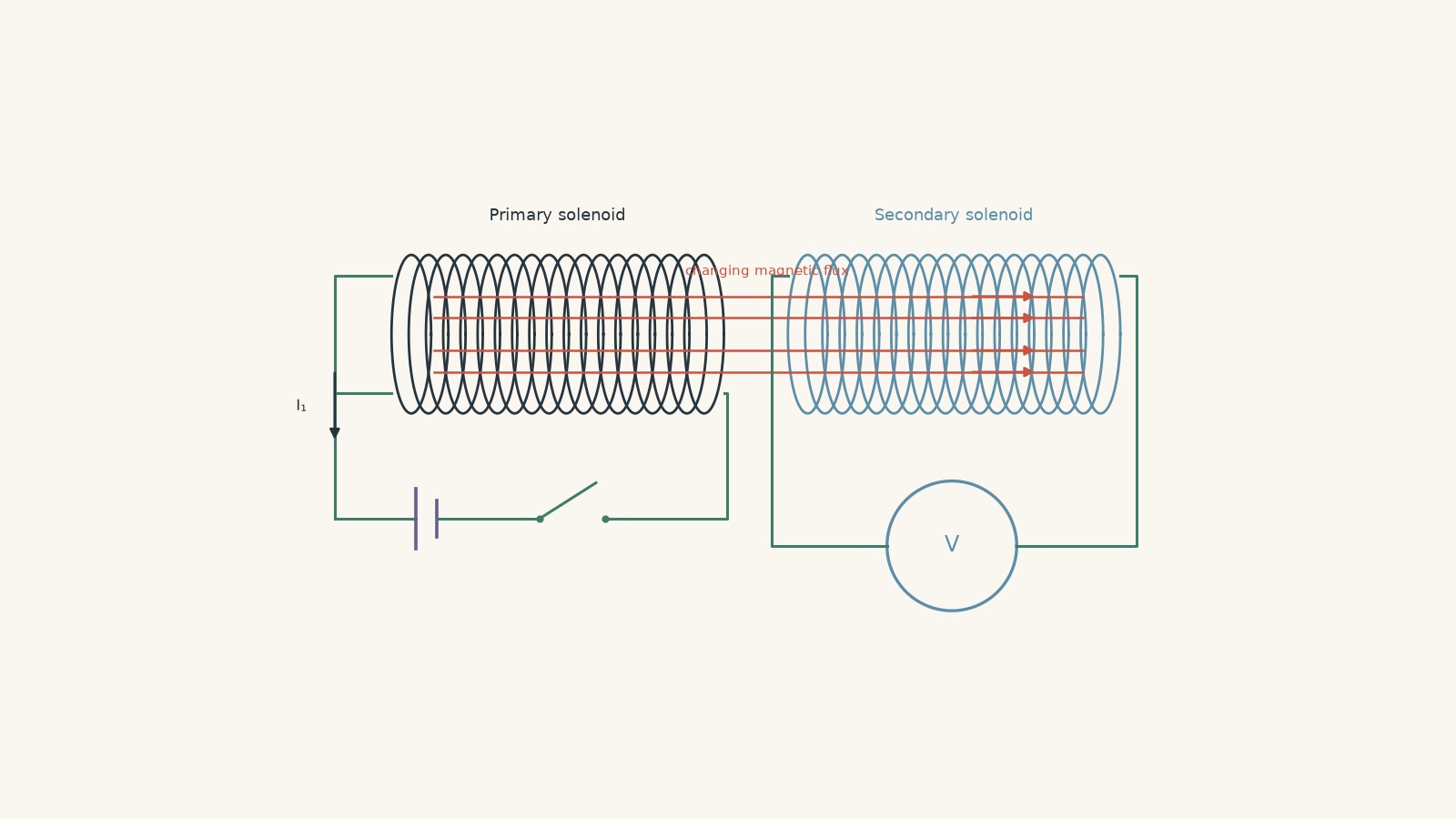
01The chain from changing current to induced emf
Call the first solenoid the primary and the second the secondary.
When current \(I_1\) flows through the primary, it creates a magnetic field \(B_1\). Some of that magnetic field passes through the turns of the secondary.
Now imagine increasing the primary current.
The sequence is:
\[ \text{changing } I_1 \rightarrow \text{changing } B_1 \rightarrow \text{changing magnetic flux through the secondary} \rightarrow \text{induced emf in the secondary} \]
That chain is worth remembering because it prevents a very common mistake. The primary current does not somehow “jump” electrically across the gap. The coils can be completely electrically isolated. What links them is the magnetic field.
A slightly silly way to remember the change part is to imagine the secondary as a friend watching your relationship status. “Still dating” for six months is not new information. “Started dating” or “broke up” causes the group chat to light up. In the same way, a steady primary current gives a steady magnetic flux, so there is no continuing induced emf. A changing current produces the interesting part.
The analogy stops there. Magnetic flux is not information being sent between coils, and an induced emf depends quantitatively on how rapidly the flux changes.
02What does “shared magnetic flux” mean?
Magnetic flux measures how much magnetic field passes through an area.
For a uniform magnetic field,
\[ \Phi = BA\cos\theta \]
where:
- \(\Phi\) is magnetic flux, measured in webers, \(\mathrm{Wb}\)
- \(B\) is magnetic field strength, measured in teslas, \(\mathrm{T}\)
- \(A\) is the area enclosed by one turn, measured in \(\mathrm{m^2}\)
- \(\theta\) is the angle between the magnetic field and the normal to the coil
If the field points straight through the face of the coil, \(\theta=0^\circ\), so \(\cos\theta=1\) and the flux is maximum.
If the field lies parallel to the plane of the coil, \(\theta=90^\circ\), so the flux is zero.
If that prerequisite needs refreshing, the key geometry is covered in Magnetic Flux for HSC Physics.
For mutual induction, however, there is an extra detail: not necessarily all of the primary’s magnetic field passes through the secondary.
Picture the secondary loop as a window. Only the part of the primary’s field passing through that window contributes to the flux through the secondary. Moving the coils apart, changing their angle, or allowing much of the primary field to miss the secondary reduces the shared flux.
Field lines are useful for picturing this, but they are not physical strings. “More field lines through the coil” is shorthand for greater magnetic flux.
03Faraday’s law gives the induced emf
Suppose the magnetic flux from the primary through each turn of the secondary changes by \(\Delta\Phi_{1\to2}\) during a time interval \(\Delta t\).
For a secondary containing \(N_2\) turns,
\[ \varepsilon_2=-N_2\frac{\Delta\Phi_{1\to2}}{\Delta t} \]
where \(\varepsilon_2\) is the average induced emf in volts.
The magnitude is therefore
\[ |\varepsilon_2|=N_2\left|\frac{\Delta\Phi_{1\to2}}{\Delta t}\right| \]
Three things immediately increase the magnitude of the induced emf:
- more secondary turns,
- a larger change in the shared flux per turn, and
- making that change happen in less time.
Notice what is not on that list: simply having a large, steady magnetic flux.
A primary could produce an enormous constant magnetic field and still induce zero emf in a stationary secondary.
That is Faraday’s law doing exactly what it says: induced emf depends on the rate of change of flux.
04Connecting the emf directly to changing primary current
For a reasonably long solenoid, the magnetic field near its centre can be approximated by
\[ B_1\approx\mu_0\frac{N_1}{L_1}I_1 \]
where:
- \(B_1\) is the primary magnetic field in teslas
- \(\mu_0=4\pi\times10^{-7}\ \mathrm{T\,m\,A^{-1}}\) is the permeability of free space
- \(N_1\) is the number of turns in the primary
- \(L_1\) is the primary’s length in metres
- \(I_1\) is the primary current in amperes
So, for a fixed solenoid,
\[ B_1\propto I_1 \]
Double the current and the magnetic field approximately doubles. More importantly for induction, changing the current changes the field.
If the secondary is aligned with the primary and an area \(A_{\text{link}}\) is effectively threaded by the primary field,
\[ \Phi_{1\to2}\approx B_1A_{\text{link}} \]
Combining this with Faraday’s law gives
\[ |\varepsilon_2| \approx N_2A_{\text{link}}\mu_0\frac{N_1}{L_1} \left|\frac{\Delta I_1}{\Delta t}\right| \]
This equation is useful, but only under the assumptions we just made: approximately uniform primary field, fixed geometry, aligned coils, and a clearly defined region of flux linkage.
The important physical statement is more general:
A changing primary current induces an emf in the secondary because it changes the magnetic flux linking the secondary.
05Worked example: A changing current in one solenoid
A long primary solenoid has \(800\) turns and a length of \(0.40\ \mathrm{m}\). A \(120\)-turn secondary solenoid of cross-sectional area \(3.0\times10^{-4}\ \mathrm{m^2}\) lies completely inside it and is coaxial with it.
The primary current increases uniformly from \(0\) to \(2.0\ \mathrm{A}\) in \(0.050\ \mathrm{s}\).
Calculate the magnitude of the average emf induced in the secondary. Assume the primary field is uniform over the secondary.
Step 1
\[ \frac{\Delta I_1}{\Delta t} = \frac{2.0-0}{0.050} = 40\ \mathrm{A\,s^{-1}} \]
Step 2
For the primary,
\[ B_1=\mu_0\frac{N_1}{L_1}I_1 \]
so
\[ \frac{\Delta B_1}{\Delta t} = \mu_0\frac{N_1}{L_1}\frac{\Delta I_1}{\Delta t} \]
Substituting,
\[ \frac{\Delta B_1}{\Delta t} = (4\pi\times10^{-7}) \left(\frac{800}{0.40}\right) (40) = 0.1005\ \mathrm{T\,s^{-1}} \]
Step 3
Because the secondary is aligned with the field,
\[ \frac{\Delta\Phi}{\Delta t} = A\frac{\Delta B_1}{\Delta t} \]
Therefore,
\[ \frac{\Delta\Phi}{\Delta t} = (3.0\times10^{-4})(0.1005) = 3.02\times10^{-5}\ \mathrm{Wb\,s^{-1}} \]
per turn.
Step 4
\[ |\varepsilon_2| = N_2\left|\frac{\Delta\Phi}{\Delta t}\right| = 120(3.02\times10^{-5}) = 3.62\times10^{-3}\ \mathrm{V} \]
So,
\[ |\varepsilon_2|\approx3.6\ \mathrm{mV} \]
The result is small, but the important point is that the secondary has an emf despite having no electrical connection to the primary.
If the primary’s field through the secondary is increasing towards the right, the secondary’s induced current, if its circuit is closed, produces a field towards the left.
06The minus sign: Lenz’s law
The minus sign in Faraday’s law tells us the direction of the induced effect.
Suppose the primary magnetic field through the secondary points to the right and is becoming stronger.
What should the secondary do?
It produces a magnetic field towards the left. That induced field opposes the increase in magnetic flux.
Now suppose the primary field still points right, but is becoming weaker.
A common mistake is to say, “The secondary must produce a field to the left because induced fields oppose the original field.”
That is not Lenz’s law.
The secondary now produces a field towards the right. It is trying to oppose the decrease by maintaining the flux that is disappearing.
So the useful rule is:
- flux increasing in one direction → induced field points the other way;
- flux decreasing in one direction → induced field points the same way.
The induced effect opposes the change in flux, not automatically the magnetic field itself.
Once you know the required induced magnetic-field direction, use the right-hand coil rule to determine the induced current direction.
07Emf is not the same thing as current
Imagine connecting only a high-resistance voltmeter across the secondary.
Faraday’s law still predicts an induced emf. The voltmeter can detect a potential difference even though almost no current flows.
If the secondary is instead connected in a closed conducting circuit, the induced emf can drive a current. For a simple resistance \(R_2\),
\[ I_2=\frac{\varepsilon_2}{R_2} \]
So these are separate questions:
- Is an emf induced?
- If the circuit is closed, how much current does that emf produce?
Do not write “no current, therefore no induction”. An open secondary can have an induced emf while carrying essentially no current.
08Not all of a large secondary necessarily helps
Our first worked example deliberately made the secondary fit completely inside the approximately uniform field of the primary.
Now change the geometry.
For an ideal long solenoid, the field is approximately uniform inside the solenoid and very small outside it. Suppose a secondary loop is much wider than the primary.
Would using the entire secondary area in \(\Phi=BA\) be sensible?
No. Much of that extra area contains almost no primary magnetic field. The useful area is approximately the region actually threaded by the primary field.
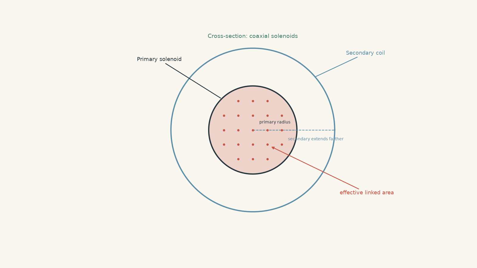
Worked example: A secondary wider than the primary
A long primary solenoid has \(1200\) turns, length \(0.60\ \mathrm{m}\), and radius \(1.2\ \mathrm{cm}\). A \(250\)-turn secondary of radius \(2.0\ \mathrm{cm}\) surrounds it coaxially.
The primary current falls uniformly from \(3.0\ \mathrm{A}\) to \(0.50\ \mathrm{A}\) in \(0.010\ \mathrm{s}\).
Estimate the magnitude of the induced emf. Treat the primary as an ideal long solenoid, with negligible field outside it.
Step 1
The tempting choice is the secondary’s area. That would be wrong under the ideal-solenoid model because the additional area outside the primary contains negligible field.
Use the primary’s cross-sectional area:
\[ A_{\text{link}} = \pi r_1^2 = \pi(0.012)^2 = 4.52\times10^{-4}\ \mathrm{m^2} \]
Step 2
\[ \frac{\Delta I_1}{\Delta t} = \frac{0.50-3.0}{0.010} = -250\ \mathrm{A\,s^{-1}} \]
The negative sign means the current is decreasing.
Step 3
\[ \frac{\Delta B_1}{\Delta t} = \mu_0\frac{N_1}{L_1}\frac{\Delta I_1}{\Delta t} \]
\[ = (4\pi\times10^{-7}) \left(\frac{1200}{0.60}\right) (-250) = -0.628\ \mathrm{T\,s^{-1}} \]
Step 4
\[ |\varepsilon_2| = N_2A_{\text{link}} \left|\frac{\Delta B_1}{\Delta t}\right| \]
\[ = 250(4.52\times10^{-4})(0.628) = 7.11\times10^{-2}\ \mathrm{V} \]
Therefore,
\[ |\varepsilon_2|\approx0.071\ \mathrm{V} \]
or about \(71\ \mathrm{mV}\).
Because the primary field is decreasing, the secondary’s induced field points in the same direction as the original primary field. It is opposing the decrease in flux.
The larger secondary still works, but its extra area beyond the primary does not magically collect flux that is not there.
09What happens when you use DC and AC?
Suppose the primary is connected to a DC supply through a switch.
When the switch first closes, the current rises from zero. That changing current creates changing flux, so the secondary gets a brief induced emf.
Once the primary current becomes constant,
\[ \frac{\Delta I_1}{\Delta t}=0 \]
so, with fixed geometry,
\[ \frac{\Delta\Phi}{\Delta t}=0 \]
and the secondary emf falls to zero.
When the switch opens, the primary current falls back towards zero. The flux now changes in the opposite sense, so the secondary receives another pulse with the opposite polarity.
An AC supply behaves differently. Its current is continually changing, so its magnetic field and shared flux also continually change. The secondary therefore experiences a continuing alternating emf.
That is the basic physics underneath a transformer.
10The mistakes worth catching
| Tempting prediction | What actually matters |
|---|---|
| A bigger primary current always means a bigger induced emf. | For fixed geometry, the induced emf depends on how quickly the current changes, not simply how large the current is. |
| A steady magnetic field keeps inducing an emf. | A steady flux produces no emf. Flux must change. |
| The induced magnetic field always opposes the primary field. | It opposes the change in flux. If primary flux is decreasing, the induced field can point in the same direction as the primary field. |
| Every bit of primary flux links the secondary. | Only the flux passing through the secondary turns contributes. Real coils can have incomplete flux linkage. |
| Making the secondary loop bigger must increase the emf. | Extra area helps only if significant magnetic field actually passes through it. |
| No secondary current means no induction. | An open circuit can have an induced emf even when essentially no current flows. |
A reliable HSC decision rule is to begin with the secondary, not the primary:
Is the magnetic flux through the secondary changing? If yes, an emf is induced. Then use the rate of change for magnitude and Lenz’s law for direction.
11Questions and solutions
Question 1
A \(200\)-turn secondary coil experiences magnetic flux from a nearby primary solenoid. The flux through each secondary turn decreases uniformly from \(5.0\times10^{-5}\ \mathrm{Wb}\) to \(1.0\times10^{-5}\ \mathrm{Wb}\) in \(0.020\ \mathrm{s}\).
Calculate the magnitude of the average induced emf.
If the original primary flux points into the page, determine the direction of the induced magnetic field and the conventional current in the secondary as viewed on the page.
Solution 1
The average induced emf is \(0.40\ \mathrm{V}\), and the induced field points into the page, requiring a clockwise conventional current.
Faraday’s law gives
\[ |\varepsilon| = N\left|\frac{\Delta\Phi}{\Delta t}\right| \]
The change in flux per turn is
\[ \Delta\Phi = 1.0\times10^{-5}-5.0\times10^{-5} = -4.0\times10^{-5}\ \mathrm{Wb} \]
Therefore,
\[ |\varepsilon| = 200 \left| \frac{-4.0\times10^{-5}}{0.020} \right| = 0.40\ \mathrm{V} \]
The primary flux into the page is decreasing. Lenz’s law says the secondary must oppose that decrease, so its induced magnetic field also points into the page.
Using the right-hand coil rule, a clockwise current produces a field into the page.
The tempting mistake is to make the induced field point out of the page because it “opposes the primary”. It does not oppose the primary field itself. It opposes the primary field becoming weaker.
Question 2
A primary solenoid and secondary solenoid are fixed in position.
When a switch is closed, the primary current rises uniformly from \(0\) to \(1.5\ \mathrm{A}\) in \(40\ \mathrm{ms}\). It then remains constant at \(1.5\ \mathrm{A}\) for \(2.0\ \mathrm{s}\). When the switch is opened, the current falls uniformly from \(1.5\ \mathrm{A}\) to zero in \(5.0\ \mathrm{ms}\).
Assume the magnetic flux linking the secondary is directly proportional to the primary current.
A galvanometer connected to the secondary deflects to the right while the switch is being closed.
Describe the galvanometer reading during the constant-current interval and when the switch is opened. Compare the magnitude of the opening pulse with the closing pulse.
Solution 2
The galvanometer reads zero while the primary current is constant, then deflects to the left when the switch is opened; the opening pulse has eight times the magnitude of the closing pulse under the stated assumptions.
During switch-on,
\[ \left|\frac{\Delta I}{\Delta t}\right| = \frac{1.5}{0.040} = 37.5\ \mathrm{A\,s^{-1}} \]
During the constant-current interval,
\[ \frac{\Delta I}{\Delta t}=0 \]
Because the geometry is fixed and flux is proportional to current,
\[ \frac{\Delta\Phi}{\Delta t}=0 \]
so there is no induced emf and the galvanometer returns to zero.
When the switch opens,
\[ \left|\frac{\Delta I}{\Delta t}\right| = \frac{1.5}{0.0050} = 300\ \mathrm{A\,s^{-1}} \]
Therefore,
\[ \frac{|\varepsilon_{\text{open}}|} {|\varepsilon_{\text{close}}|} = \frac{300}{37.5} = 8 \]
The opening change is in the opposite direction, so Lenz’s law gives the opposite polarity and hence a deflection to the left.
A tempting argument is that the strongest induction should occur while the current is sitting at its maximum value of \(1.5\ \mathrm{A}\). The actual constraint is Faraday’s law: once that current stops changing, the shared magnetic flux stops changing too.
Question 3
A long primary solenoid has \(1000\) turns, length \(0.50\ \mathrm{m}\), and radius \(1.0\ \mathrm{cm}\). A coaxial secondary has \(300\) turns and radius \(2.0\ \mathrm{cm}\), completely surrounding the primary.
The primary current increases at a constant rate of \(25\ \mathrm{A\,s^{-1}}\).
Assume the magnetic field is uniform inside the primary and zero outside it.
Calculate the magnitude of the emf induced in the secondary. If the increasing primary field points to the left, state the direction of the secondary’s induced field.
Solution 3
The induced emf is approximately \(5.9\ \mathrm{mV}\), and the secondary’s induced magnetic field points to the right.
The first trap is the area. Although the secondary radius is \(2.0\ \mathrm{cm}\), the model says the primary field exists only inside the primary radius of \(1.0\ \mathrm{cm}\).
Therefore,
\[ A_{\text{link}} = \pi(0.010)^2 = 3.14\times10^{-4}\ \mathrm{m^2} \]
The rate of change of primary magnetic field is
\[ \frac{\Delta B}{\Delta t} = \mu_0\frac{N_1}{L_1} \frac{\Delta I_1}{\Delta t} \]
Substituting,
\[ \frac{\Delta B}{\Delta t} = (4\pi\times10^{-7}) \left(\frac{1000}{0.50}\right) (25) = 6.28\times10^{-2}\ \mathrm{T\,s^{-1}} \]
Faraday’s law then gives
\[ |\varepsilon_2| = N_2A_{\text{link}} \left|\frac{\Delta B}{\Delta t}\right| \]
\[ = 300(3.14\times10^{-4})(6.28\times10^{-2}) = 5.92\times10^{-3}\ \mathrm{V} \]
So,
\[ |\varepsilon_2|\approx5.9\ \mathrm{mV} \]
The primary field points left and is becoming stronger. The induced secondary field must therefore point right to oppose that increase.
The tempting route is to calculate \(BA\) using the full \(2.0\ \mathrm{cm}\) secondary radius. That treats the region outside the primary as though it contains the same field as the inside, directly contradicting the model given in the question.
Question 4
A long primary solenoid has radius
\[ R=1.5\times10^{-2}\ \mathrm{m} \]
Near its centre, its magnetic field changes at a rate of
\[ \left|\frac{\Delta B}{\Delta t}\right| = 0.40\ \mathrm{T\,s^{-1}} \]
The field may be treated as uniform inside radius \(R\) and zero outside.
You have \(18.0\ \mathrm{m}\) of wire and use all of it to make a very short coaxial secondary solenoid. Every secondary turn has approximately the same radius \(r\). Ignore wire thickness, resistance, and end effects.
Determine the value of \(r\) that maximises the induced emf. Derive the dependence of emf on \(r\) for both \(r\le R\) and \(r\ge R\), then calculate the maximum emf.
Solution 4
The induced emf is maximised when the secondary radius equals the primary radius, \(r=R=1.5\ \mathrm{cm}\), giving a maximum emf of approximately \(5.4\times10^{-2}\ \mathrm{V}\).
There are two competing effects. Increasing \(r\) gives each turn more useful area at first, but because the total wire length is fixed, a larger radius also means fewer turns. Once \(r\) exceeds the primary radius, the extra enclosed area contains no field at all in the stated model.
Let the total wire length be \(L_{\mathrm w}=18.0\ \mathrm{m}\).
One circular turn requires approximately \(2\pi r\) of wire, so
\[ N=\frac{L_{\mathrm w}}{2\pi r} \]
For \(r\le R\), the entire area of each secondary turn lies within the primary field. The useful area is
\[ A=\pi r^2 \]
Therefore,
\[ |\varepsilon| = N\pi r^2\left|\frac{\Delta B}{\Delta t}\right| \]
Substituting for \(N\),
\[ |\varepsilon| = \frac{L_{\mathrm w}}{2\pi r} \pi r^2 \left|\frac{\Delta B}{\Delta t}\right| \]
so
\[ |\varepsilon| = \frac{L_{\mathrm w}r}{2} \left|\frac{\Delta B}{\Delta t}\right| \qquad (r\le R) \]
Thus the emf increases with \(r\) while \(r\le R\).
For \(r\ge R\), making the secondary wider does not add useful flux because the model specifies zero field outside the primary. The effective area is now fixed at
\[ A_{\text{link}}=\pi R^2 \]
Hence,
\[ |\varepsilon| = N\pi R^2 \left|\frac{\Delta B}{\Delta t}\right| \]
and therefore
\[ |\varepsilon| = \frac{L_{\mathrm w}R^2}{2r} \left|\frac{\Delta B}{\Delta t}\right| \qquad (r\ge R) \]
This expression decreases as \(r\) increases.
The first expression rises up to \(r=R\), while the second falls after \(r=R\). The maximum must therefore occur at the boundary:
\[ r=R=0.015\ \mathrm{m} \]
The maximum emf is
\[ |\varepsilon_{\max}| = \frac{(18.0)(0.015)}{2}(0.40) = 5.4\times10^{-2}\ \mathrm{V} \]
so
\[ |\varepsilon_{\max}|=0.054\ \mathrm{V} \]
The tempting route is to say either “more turns is always better” and make \(r\) tiny, or “more area is always better” and make \(r\) huge. Neither works because the same finite length of wire controls both quantities. The optimum appears exactly where making the loop larger stops capturing additional magnetic field.
Question 5
A secondary solenoid is near a primary solenoid. Rather than giving the detailed geometry, suppose its flux linkage is described by
\[ \Lambda=0.012fI_1 \]
where:
- \(\Lambda=N_2\Phi\) is the secondary’s flux linkage in \(\mathrm{Wb\,turn}\),
- \(I_1\) is the primary current in amperes, and
- \(f\) is the fraction describing how strongly the primary flux links the secondary.
Take positive \(\Lambda\) to mean flux in the direction produced by positive primary current.
The system passes through three consecutive \(20\ \mathrm{ms}\) intervals.
During interval A, \(f=0.80\) and the primary current rises uniformly from \(0\) to \(2.0\ \mathrm{A}\).
During interval B, the primary current remains constant at \(2.0\ \mathrm{A}\), but the secondary is moved away so that \(f\) falls uniformly from \(0.80\) to \(0.30\).
During interval C, \(f=0.30\) and the primary current falls uniformly from \(2.0\ \mathrm{A}\) to zero.
For each interval, calculate the average induced emf, including its sign according to
\[ \varepsilon=-\frac{\Delta\Lambda}{\Delta t} \]
Then find the total signed voltage-time area,
\[ \sum \varepsilon\Delta t \]
across all three intervals.
Finally, explain why interval B is the conceptual trap.
Solution 5
The average induced emfs are \(-0.96\ \mathrm{V}\) in interval A, \(+0.60\ \mathrm{V}\) in interval B, and \(+0.36\ \mathrm{V}\) in interval C. The total signed voltage-time area is zero. Interval B still has an induced emf even though the primary current is constant because the shared flux changes when the geometry changes.
Start with interval A.
Initially,
\[ \Lambda_i=0 \]
At the end,
\[ \Lambda_f = 0.012(0.80)(2.0) = 0.0192\ \mathrm{Wb\,turn} \]
Therefore,
\[ \varepsilon_A = -\frac{0.0192-0}{0.020} = -0.96\ \mathrm{V} \]
The negative sign expresses Lenz’s law: the primary-linked flux is increasing positively, so the induced emf acts in the opposing sense.
For interval B, the current stays at \(2.0\ \mathrm{A}\), but \(f\) changes.
The initial linkage is
\[ \Lambda_i = 0.012(0.80)(2.0) = 0.0192\ \mathrm{Wb\,turn} \]
The final linkage is
\[ \Lambda_f = 0.012(0.30)(2.0) = 0.0072\ \mathrm{Wb\,turn} \]
Hence,
\[ \varepsilon_B = -\frac{0.0072-0.0192}{0.020} = +0.60\ \mathrm{V} \]
For interval C,
\[ \Lambda_i=0.0072\ \mathrm{Wb\,turn} \]
and, because the primary current ends at zero,
\[ \Lambda_f=0 \]
Thus,
\[ \varepsilon_C = -\frac{0-0.0072}{0.020} = +0.36\ \mathrm{V} \]
Now calculate the signed voltage-time areas.
\[ \varepsilon_A\Delta t = (-0.96)(0.020) = -0.0192\ \mathrm{V\,s} \]
\[ \varepsilon_B\Delta t = (0.60)(0.020) = +0.0120\ \mathrm{V\,s} \]
\[ \varepsilon_C\Delta t = (0.36)(0.020) = +0.0072\ \mathrm{V\,s} \]
Therefore,
\[ \sum\varepsilon\Delta t = -0.0192+0.0120+0.0072 = 0 \]
This is not a coincidence. Faraday’s law gives
\[ \int\varepsilon\,dt=-\Delta\Lambda \]
over the whole process. The secondary begins with zero flux linkage and eventually returns to zero flux linkage, so the total signed area must also be zero.
Interval B is the hinge. A student who memorises “changing current causes induction” may predict zero emf because \(I_1\) is constant. But changing current is only one way to change magnetic flux.
The deeper rule is that the shared magnetic flux must change.
Moving the coils changes how much of the primary’s field links the secondary, so an emf can be induced even while the primary current itself remains steady.
12From mutual induction to transformers
Two nearby solenoids already contain the essential transformer physics. A changing primary current creates changing magnetic flux, some of that flux links the secondary, and Faraday’s law gives the secondary emf.
A transformer makes that process far more effective. Its primary current alternates continuously, and a shared magnetic core directs much more of the changing flux through both windings. The number of turns then controls how strongly that changing flux appears as an emf in each coil.
So when transformer equations arrive, the useful picture is not “a transformer somehow changes voltage”. The underlying chain is the same one developed here:
\[ \text{changing current} \rightarrow \text{changing magnetic field} \rightarrow \text{changing shared flux} \rightarrow \text{induced emf} \]
That is the idea to carry forward when you meet turns ratios, incomplete flux linkage, and transformer efficiency.