
Magnetic Flux for HSC Physics: Using Φ = BA cos θ
Learn how magnetic flux depends on field strength, area, and angle, and how to calculate changes in flux in HSC Physics problems.
A wire loop sits in a magnetic field. The field is strong, the loop is large, and yet the magnetic flux through it can be exactly zero.
How?
Before reading on, picture a flat loop like a picture frame. If the magnetic field points straight through the middle of the frame, you would expect a large flux. Now turn the frame so the field runs along its surface instead. The same magnetic field is still there, but none of it passes through the loop.
That is the idea magnetic flux measures: how much magnetic field passes through a surface.
01Start with the physical picture
Imagine rain falling vertically onto a skylight.
A horizontal skylight catches lots of rain. Tilt it, and it catches less. Turn it completely vertical, and almost no rain passes through its opening.
Magnetic flux behaves similarly. The magnetic field is the “rain”, and the loop provides the surface we are interested in.
There is one important limit to this analogy. Magnetic field lines are not physical streams of particles flowing through the loop. They are a way of representing a magnetic field. Flux is a mathematical measure of how much of that field passes through a chosen surface.
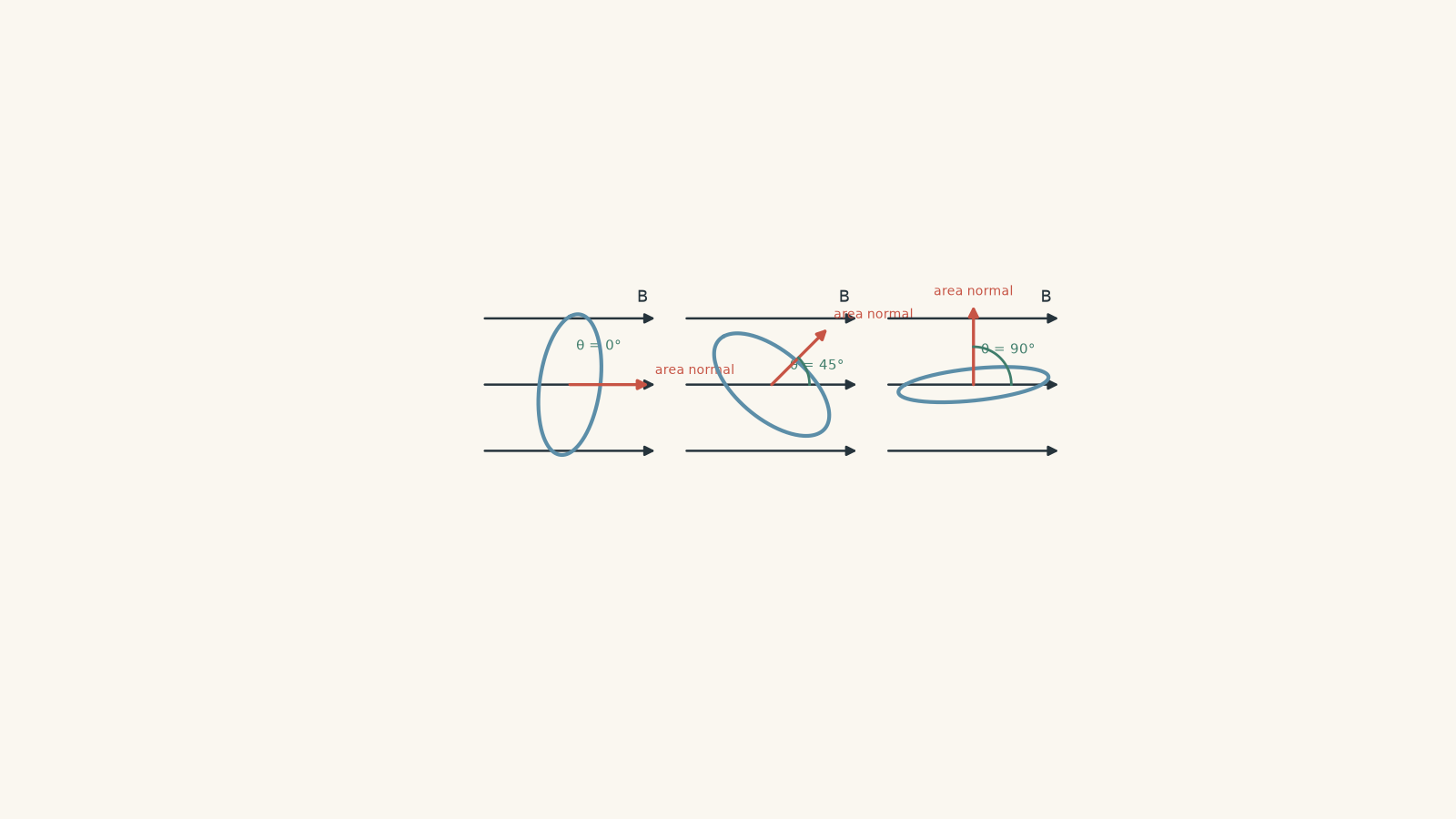
Suppose all three loops have the same area and sit in the same magnetic field.
Which should have the greatest magnetic flux?
The first one, where the field passes directly through the loop. The tilted loop has less flux, and the loop with the field running along its surface has zero flux.
That tells us magnetic flux depends on more than just magnetic field strength.
02The magnetic flux equation
For a flat surface in a uniform magnetic field,
\[ \Phi = BA\cos\theta \]
where:
- \(\Phi\) is magnetic flux, measured in webers, \(\text{Wb}\)
- \(B\) is magnetic flux density, measured in tesla, \(\text{T}\)
- \(A\) is the area of the surface, measured in square metres, \(\text{m}^2\)
- \(\theta\) is the angle between the magnetic field and the normal to the surface
The last point causes more mistakes than the rest of the equation combined.
The angle is measured from the normal
The normal is an imaginary line drawn at \(90^\circ\) to the surface.
So if a magnetic field passes straight through a loop, the field is parallel to the normal.
That means
\[ \theta = 0^\circ \]
and therefore
\[ \Phi = BA\cos 0^\circ = BA \]
The flux is at its maximum magnitude.
If the magnetic field runs along the plane of the loop, it is perpendicular to the normal. Then
\[ \theta = 90^\circ \]
so
\[ \Phi = BA\cos 90^\circ = 0 \]
There is no magnetic flux through the surface.
A student will sometimes reason, “The field is at \(90^\circ\) to the loop, so I should use \(90^\circ\).” That sounds sensible because everyday language encourages us to compare the field with the surface itself.
The equation doesn’t do that. It compares the field with the normal.
A useful habit is to draw the normal before writing down \(\theta\).
03Why does the cosine appear?
Rather than memorising the cosine, we can see where it comes from.
Suppose the loop is tilted. The magnetic field no longer passes straight through the full effective area of the loop.
From the field’s point of view, the loop behaves as though it has a smaller area:
\[ A_{\perp} = A\cos\theta \]
where \(A_{\perp}\) is the area effectively perpendicular to the magnetic field.
The flux is then
\[ \Phi = B A_{\perp} \]
so
\[ \Phi = BA\cos\theta \]
This is why increasing \(\theta\) from \(0^\circ\) towards \(90^\circ\) reduces the flux.
The loop itself has not physically shrunk. Its effective area relative to the field has changed.
Worked example: Finding the flux through a tilted loop
A rectangular loop has an area of \(0.080\,\text{m}^2\). It is placed in a uniform magnetic field of \(0.35\,\text{T}\). The normal to the loop makes an angle of \(40^\circ\) with the magnetic field. Calculate the magnetic flux through the loop.
Step 1
\[ B = 0.35\,\text{T}, \qquad A = 0.080\,\text{m}^2, \qquad \theta = 40^\circ \]
Step 2
\[ \Phi = BA\cos\theta \]
Step 3
\[ \Phi = (0.35)(0.080)\cos 40^\circ \]
\[ \Phi = 2.14\times10^{-2}\,\text{Wb} \]
The magnetic flux is approximately
\[ \Phi = 0.021\,\text{Wb} \]
The maximum possible flux for this loop would be \(BA = 0.028\,\text{Wb}\). Tilting the loop to \(40^\circ\) reduces the amount of field passing through its effective area.
04Three ways magnetic flux can change
The equation
\[ \Phi = BA\cos\theta \]
shows three direct ways to change magnetic flux.
Change the magnetic field strength
If \(A\) and \(\theta\) stay constant, increasing \(B\) increases the flux.
For example, doubling \(B\) doubles \(\Phi\).
If a \(0.020\,\text{m}^2\) loop is perpendicular to a field so that \(\theta=0^\circ\), then changing the field from \(0.10\,\text{T}\) to \(0.30\,\text{T}\) changes the flux from
\[ \Phi_i=(0.10)(0.020)=2.0\times10^{-3}\,\text{Wb} \]
to
\[ \Phi_f=(0.30)(0.020)=6.0\times10^{-3}\,\text{Wb} \]
The change in flux is
\[ \Delta\Phi=\Phi_f-\Phi_i \]
\[ \Delta\Phi=4.0\times10^{-3}\,\text{Wb} \]
Change the area exposed to the field
A larger area can have a larger magnetic flux.
This does not always mean physically stretching the loop. A loop can move into or out of a region containing a magnetic field, so the area actually inside the field changes.
Suppose only half of a flat loop lies inside a uniform magnetic field. If the field is zero outside that region, you cannot simply use the full loop area in \(\Phi=BA\cos\theta\).
You use the area through which the relevant field actually passes.
That distinction becomes important in induction problems involving a loop entering or leaving a magnetic field.
Change the angle
Even if \(B\) and \(A\) remain constant, rotating the loop changes \(\theta\), which changes \(\cos\theta\).
For a fixed loop and field:
| \(\theta\) | \(\cos\theta\) | Flux |
|---|---|---|
| \(0^\circ\) | \(1\) | maximum positive value |
| \(30^\circ\) | \(0.866\) | slightly reduced |
| \(60^\circ\) | \(0.500\) | half the maximum |
| \(90^\circ\) | \(0\) | zero |
| \(120^\circ\) | \(-0.500\) | negative |
| \(180^\circ\) | \(-1\) | maximum magnitude, opposite sign |
The negative values need some care.
05What does negative magnetic flux mean?
A surface has two possible normal directions. Once we choose one as positive, a magnetic field pointing partly in that direction gives positive flux. A field passing through the surface in the opposite sense gives negative flux.
Negative flux does not mean “less magnetic field exists”.
It tells us the field passes through the chosen surface in the opposite direction.
For many simple HSC calculations, you may mainly care about the magnitude. But the sign becomes important when tracking changes in flux.
For example, suppose a loop rotates from
\[ \theta_i=0^\circ \]
to
\[ \theta_f=180^\circ \]
with \(B\) and \(A\) constant.
Initially,
\[ \Phi_i=BA \]
and finally,
\[ \Phi_f=-BA \]
So the change in flux is
\[ \Delta\Phi=\Phi_f-\Phi_i=-BA-BA=-2BA \]
Its magnitude is \(2BA\), not zero.
A tempting argument is, “The loop starts and finishes with the same maximum amount of field passing through it.”
The missing detail is direction. The flux has reversed sign.
Worked example: A rotating loop
A single loop of area \(0.050\,\text{m}^2\) is in a uniform magnetic field of \(0.80\,\text{T}\). Its normal initially makes an angle of \(20^\circ\) with the field. The loop is rotated so that its normal makes an angle of \(110^\circ\) with the field.
Calculate the initial flux, final flux, and change in flux.
Step 1
\[ \Phi_i=BA\cos\theta_i \]
\[ \Phi_i=(0.80)(0.050)\cos20^\circ \]
\[ \Phi_i=3.76\times10^{-2}\,\text{Wb} \]
Step 2
\[ \Phi_f=BA\cos\theta_f \]
\[ \Phi_f=(0.80)(0.050)\cos110^\circ \]
\[ \Phi_f=-1.37\times10^{-2}\,\text{Wb} \]
Step 3
\[ \Delta\Phi=\Phi_f-\Phi_i \]
\[ \Delta\Phi=(-1.37\times10^{-2})-(3.76\times10^{-2}) \]
\[ \Delta\Phi=-5.13\times10^{-2}\,\text{Wb} \]
So the flux changes by
\[ \Delta\Phi=-0.0513\,\text{Wb} \]
or by a magnitude of \(0.0513\,\text{Wb}\).
The negative sign tells us the final flux is lower according to our chosen normal direction. More importantly, the loop has crossed through zero flux and ended with the field passing through it in the opposite sense.
06Magnetic flux is not magnetic field strength
Magnetic flux \(\Phi\) and magnetic flux density \(B\) are related, but they are not the same quantity.
A \(2.0\,\text{T}\) magnetic field can produce zero flux through a particular loop if the field runs along the plane of the loop.
Meanwhile, a weaker field can produce non-zero flux if it passes through a suitably oriented surface.
So this statement is wrong:
A larger magnetic field always means a larger magnetic flux.
It is only true when the relevant area and orientation are unchanged.
A better decision rule is to inspect all three factors:
\[ B,\qquad A,\qquad \cos\theta \]
If any of them changes, the flux may change.
07Be careful with coils containing several turns
Magnetic flux \(\Phi\) refers to the flux through one surface.
If a coil contains \(N\) identical turns and the same flux passes through every turn, the total flux linkage is
\[ N\Phi \]
That distinction becomes important in electromagnetic induction.
For example, if each turn has a flux of \(2.0\times10^{-3}\,\text{Wb}\) and the coil has \(50\) turns, then the flux through each turn remains
\[ 2.0\times10^{-3}\,\text{Wb} \]
while the flux linkage is
\[ N\Phi=(50)(2.0\times10^{-3})=0.100\,\text{Wb-turn} \]
Adding turns has not magically increased \(B\), the loop area, or the flux through one turn.
It has increased how many turns experience that flux.
08Where \(\Phi=BA\cos\theta\) stops being enough
The simple equation assumes the magnetic field is uniform across a flat surface.
If different parts of a surface experience different magnetic field strengths or directions, one value of \(B\) and one value of \(\theta\) cannot describe the whole surface exactly.
The deeper idea is still the same: magnetic flux depends on the component of the magnetic field passing through each part of the surface.
For HSC-style uniform-field problems, \(\Phi=BA\cos\theta\) does that job directly.
09Questions and solutions
Question 1
A flat loop of area \(0.030\,\text{m}^2\) is placed in a uniform \(0.50\,\text{T}\) magnetic field. The magnetic field is parallel to the normal of the loop.
Calculate the magnetic flux through the loop.
Solution 1
The magnetic flux is \(1.5\times10^{-2}\,\text{Wb}\).
Because the magnetic field is parallel to the normal,
\[ \theta=0^\circ \]
Use
\[ \Phi=BA\cos\theta \]
Substituting,
\[ \Phi=(0.50)(0.030)\cos0^\circ \]
\[ \Phi=0.015\,\text{Wb} \]
So
\[ \boxed{\Phi=1.5\times10^{-2}\,\text{Wb}} \]
The tempting mistake is to say the field is at \(90^\circ\) to the surface and substitute \(90^\circ\). The angle in the flux equation is measured from the normal, not from the plane of the loop.
Question 2
A loop of area \(0.12\,\text{m}^2\) is placed in a uniform magnetic field. The field strength increases from \(0.25\,\text{T}\) to \(0.70\,\text{T}\) while the angle between the field and the loop’s normal changes from \(30^\circ\) to \(60^\circ\).
Calculate the initial flux, final flux, and change in flux. State whether the increase in magnetic field strength guarantees that the flux increases.
Solution 2
The flux increases from approximately \(0.0260\,\text{Wb}\) to \(0.0420\,\text{Wb}\), giving \(\Delta\Phi\approx0.0160\,\text{Wb}\). An increase in \(B\) does not, by itself, guarantee an increase in flux.
Initially,
\[ \Phi_i=B_iA\cos\theta_i \]
\[ \Phi_i=(0.25)(0.12)\cos30^\circ \]
\[ \Phi_i=2.60\times10^{-2}\,\text{Wb} \]
Finally,
\[ \Phi_f=B_fA\cos\theta_f \]
\[ \Phi_f=(0.70)(0.12)\cos60^\circ \]
\[ \Phi_f=4.20\times10^{-2}\,\text{Wb} \]
Therefore,
\[ \Delta\Phi=\Phi_f-\Phi_i \]
\[ \Delta\Phi=(4.20-2.60)\times10^{-2} \]
\[ \Delta\Phi=1.60\times10^{-2}\,\text{Wb} \]
The tempting route is to look only at \(B\) and conclude immediately that the flux must rise because the magnetic field became stronger.
But
\[ \Phi=BA\cos\theta \]
depends on both \(B\) and \(\theta\). Here, increasing the angle reduces \(\cos\theta\), partly cancelling the effect of the stronger magnetic field. The increase in \(B\) happens to be large enough that the final flux is still greater.
In a different numerical case, the field could become stronger while the flux decreases.
Question 3
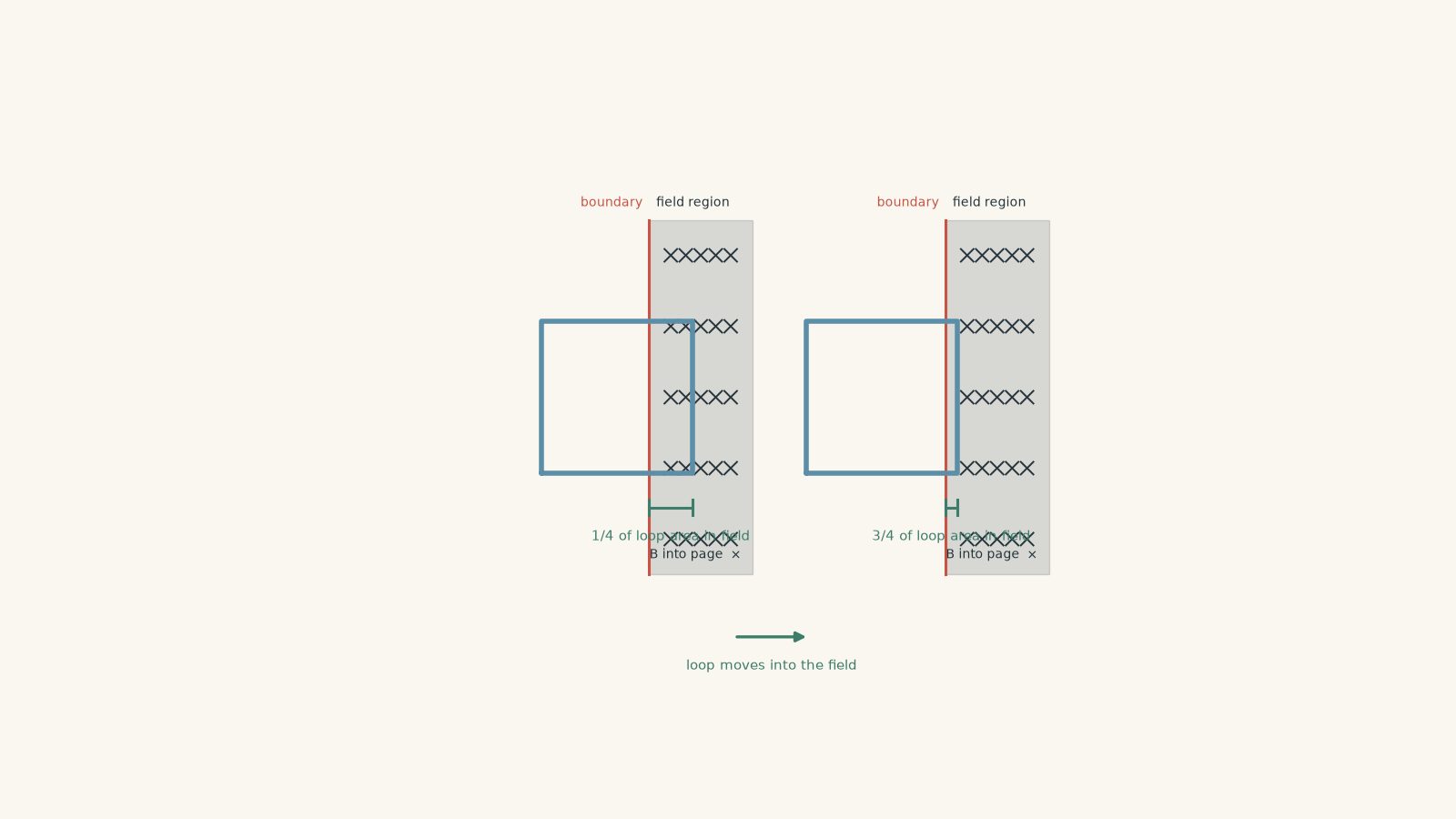
A square loop has side length \(0.20\,\text{m}\). It lies partly inside a region containing a uniform magnetic field of \(0.60\,\text{T}\). The field is perpendicular to the plane of the loop.
Initially, one-quarter of the loop’s area is inside the field. The loop then moves without rotating until three-quarters of its area is inside the field.
Calculate the change in magnetic flux.
Solution 3
The magnetic flux increases by \(0.012\,\text{Wb}\).
The full loop area is
\[ A=(0.20)^2=0.040\,\text{m}^2 \]
The field is perpendicular to the plane, so it is parallel to the normal and
\[ \theta=0^\circ \]
Initially, only one-quarter of the loop is inside the field:
\[ A_i=\frac14(0.040)=0.010\,\text{m}^2 \]
Therefore,
\[ \Phi_i=BA_i\cos0^\circ \]
\[ \Phi_i=(0.60)(0.010)=0.0060\,\text{Wb} \]
Finally,
\[ A_f=\frac34(0.040)=0.030\,\text{m}^2 \]
so
\[ \Phi_f=(0.60)(0.030)=0.018\,\text{Wb} \]
The change is
\[ \Delta\Phi=\Phi_f-\Phi_i \]
\[ \Delta\Phi=0.018-0.0060 \]
\[ \boxed{\Delta\Phi=0.012\,\text{Wb}} \]
The tempting mistake is to use the entire \(0.040\,\text{m}^2\) area in both positions. That would predict no change in flux because \(B\), the loop’s total area, and its orientation have not changed.
The missing constraint is that the magnetic field exists only in part of the region. The effective area experiencing the field changes as the loop crosses the boundary.
Question 4
A loop of fixed area \(A\) is in a uniform magnetic field. Initially, the field has magnitude \(B\) and is parallel to the loop’s normal.
The loop is then rotated to an angle of \(60^\circ\) to the field while the field strength is simultaneously doubled.
A student argues:
“Rotating the loop to \(60^\circ\) halves its flux, but doubling \(B\) doubles it again, so the final flux must equal the initial flux.”
Is the student correct? Then determine what happens if the loop is instead rotated to \(120^\circ\) while the field is doubled.
Solution 4
The student is correct for \(60^\circ\), but the \(120^\circ\) case has the same flux magnitude and the opposite sign.
Initially,
\[ \Phi_i=BA\cos0^\circ=BA \]
For the first final state,
\[ B_f=2B \]
and
\[ \theta_f=60^\circ \]
Therefore,
\[ \Phi_f=(2B)A\cos60^\circ \]
Since
\[ \cos60^\circ=\frac12 \]
we obtain
\[ \Phi_f=(2B)A\left(\frac12\right)=BA \]
So the flux is unchanged:
\[ \Delta\Phi=0 \]
The student’s reasoning works in this case.
Now consider \(120^\circ\):
\[ \Phi_f=(2B)A\cos120^\circ \]
and
\[ \cos120^\circ=-\frac12 \]
so
\[ \Phi_f=-BA \]
The final flux has the same magnitude as the initial flux but the opposite sign.
Therefore,
\[ \Delta\Phi=\Phi_f-\Phi_i \]
\[ \Delta\Phi=-BA-BA \]
\[ \boxed{\Delta\Phi=-2BA} \]
The tempting route is to use only the magnitude of \(\cos120^\circ\), treating \(120^\circ\) as though it were equivalent to \(60^\circ\).
Geometrically, the effective area magnitude is the same. Directionally, however, the magnetic field now passes through the chosen surface in the opposite sense. That sign reversal completely changes \(\Delta\Phi\).
Question 5
Two identical flat loops, X and Y, each have area \(A\).
Loop X is in a uniform magnetic field of magnitude \(B\). Its normal initially points in the same direction as the field. It is rotated through \(90^\circ\).
Loop Y is in a uniform magnetic field of magnitude \(2B\). Its normal initially makes an angle of \(60^\circ\) with the field. It is then rotated through \(60^\circ\) in the same rotational sense, so its final angle is \(120^\circ\).
A student claims that Y must have the greater change in magnetic flux because it is in the stronger magnetic field and rotates through a substantial angle.
Determine the change in flux for each loop and compare their magnitudes.
Solution 5
The two loops have exactly the same magnitude of change in magnetic flux, \(BA\), even though loop Y is in twice the magnetic field.
For loop X, the initial flux is
\[ \Phi_{Xi}=BA\cos0^\circ=BA \]
After rotation through \(90^\circ\),
\[ \Phi_{Xf}=BA\cos90^\circ=0 \]
Therefore,
\[ \Delta\Phi_X=\Phi_{Xf}-\Phi_{Xi} \]
\[ \Delta\Phi_X=0-BA=-BA \]
so
\[ |\Delta\Phi_X|=BA \]
Now consider loop Y.
Its magnetic field strength is \(2B\), and its initial angle is \(60^\circ\):
\[ \Phi_{Yi}=(2B)A\cos60^\circ \]
\[ \Phi_{Yi}=(2B)A\left(\frac12\right)=BA \]
Its final angle is \(120^\circ\):
\[ \Phi_{Yf}=(2B)A\cos120^\circ \]
\[ \Phi_{Yf}=(2B)A\left(-\frac12\right)=-BA \]
Therefore,
\[ \Delta\Phi_Y=\Phi_{Yf}-\Phi_{Yi} \]
\[ \Delta\Phi_Y=-BA-BA=-2BA \]
So
\[ |\Delta\Phi_Y|=2BA \]
Therefore, loop Y actually has twice the magnitude of flux change:
\[ \boxed{|\Delta\Phi_Y|=2|\Delta\Phi_X|} \]
The tempting first comparison is still incomplete, though. Saying “Y has a stronger magnetic field” is not enough to establish the result. Nor is comparing the rotation angles alone.
The decisive feature is that loop Y crosses from positive flux to negative flux. Its flux changes from \(+BA\) to \(-BA\), so the total change spans \(2BA\).
Loop X changes only from \(+BA\) to zero.
This is why flux problems are safest when you calculate the initial and final signed values separately:
\[ \Delta\Phi=\Phi_f-\Phi_i \]
rather than trying to judge the change from how far the loop rotates.
10What magnetic flux lets you understand next
Magnetic flux becomes especially useful when it changes.
A changing \(B\), a changing exposed area, or a changing angle can all produce a changing \(\Phi\). That gives us one common way to describe apparently different situations: moving a loop into a magnetic field, rotating a coil, or changing the field itself.
The next step is Faraday’s law. It connects the rate of change of magnetic flux to an induced emf. At that point, it will no longer be enough to ask, “What is the flux?” You will need to ask, “How much does the flux change, and how quickly does that change happen?”