
Electric Fields Between Parallel Plates: Using E = V/d
Learn how to calculate electric field strength between parallel plates, determine field direction, and recognise when the uniform-field model breaks down.
Two metal plates are 20 mm apart. One is at \(+600\ \text{V}\), and the other is at \(0\ \text{V}\). Put an electron between them and it accelerates towards the positive plate.
Now make the gap twice as large but keep the same 600 V potential difference. What happens to the electric field?
A tempting answer is, “Nothing – the voltage is still 600 V.” But the field becomes half as strong. The same change in electric potential is now spread across twice the distance.
That idea – voltage change per unit distance – is the key to understanding electric fields between parallel plates.
01From potential difference to electric field
Picture two large, flat, parallel conducting plates:
- the positive plate is at higher electric potential,
- the negative plate is at lower electric potential,
- the plates are separated by a perpendicular distance \(d\).
In the central region between sufficiently large plates, the electric field is approximately constant in both magnitude and direction.
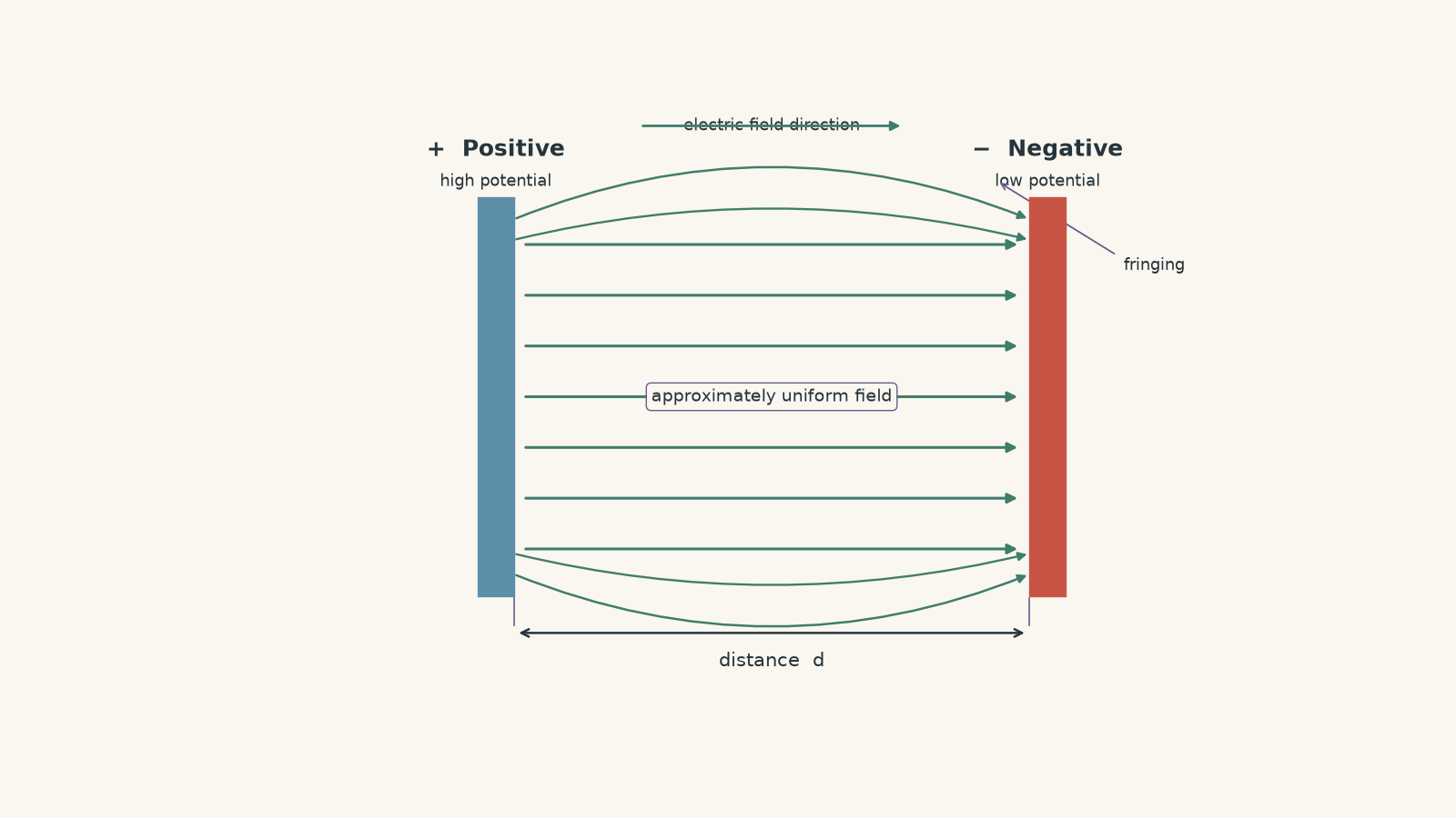
Before using an equation, imagine the voltage as a slope.
Suppose the potential falls by 600 V across 20 mm. If that same 600 V drop occurs across only 10 mm, the potential changes more rapidly with position. We say the electric field is stronger.
It is a little like a ramp. A 2 m rise spread across a long distance gives a gentle slope. The same 2 m rise squeezed into a short distance gives a steeper slope.
Here:
- the potential difference \(V\) plays the role of the change in height,
- the plate separation \(d\) plays the role of the horizontal distance,
- the electric field strength \(E\) tells us how steeply the potential changes with position.
The analogy eventually breaks. Electric potential is not literal height, and an electric field is a vector, not a physical ramp. But the “steepness” idea is useful.
For a uniform electric field between parallel plates,
\[
E=\frac{V}{d}
\]
where:
- \(E\) is the electric field strength in volts per metre, \(\text{V m}^{-1}\), or equivalently newtons per coulomb, \(\text{N C}^{-1}\),
- \(V\) is the magnitude of the potential difference between the plates in volts, \(\text{V}\),
- \(d\) is the perpendicular separation of the plates in metres, \(\text{m}\).
Notice that \(V\) here means the potential difference, not necessarily the potential of either plate individually.
A plate at \(+700\ \text{V}\) opposite a plate at \(+200\ \text{V}\) has a potential difference of
\[
700-200=500\ \text{V}.
\]
For the field magnitude, you would use \(V=500\ \text{V}\).
Worked example: Finding the field between two plates
Two parallel plates are separated by \(15\ \text{mm}\) and have a potential difference of \(450\ \text{V}\). Calculate the electric field strength between them.
Step 1
\[
d=15\ \text{mm}=0.015\ \text{m}
\]
Step 2
\[
E=\frac{V}{d}
\]
Step 3
\[
E=\frac{450}{0.015}=3.0\times10^4\ \text{V m}^{-1}
\]
So,
\[
E=3.0\times10^4\ \text{V m}^{-1}.
\]
This means the electric potential changes by \(3.0\times10^4\ \text{V}\) for every metre travelled in the field direction. We do not actually need a one-metre-wide capacitor for that interpretation to be useful. It describes the rate of potential change.
02Which way does the field point?
The equation \(E=V/d\) gives the magnitude of the field. Electric field also has direction.
By definition, the electric field points in the direction that a positive test charge would accelerate.
Between parallel plates, it therefore points:
from the positive, higher-potential plate towards the negative, lower-potential plate.
This creates a common trap with electrons.
An electron has negative charge, so the electric force on it is opposite the electric field direction.
The force on any charge is
\[
F=qE,
\]
where \(F\) is electric force in newtons, \(q\) is charge in coulombs, and \(E\) is electric field strength in newtons per coulomb.
For a positive charge, force and field point in the same direction. For a negative charge, they point in opposite directions.
So an electron between the plates accelerates towards the positive plate even though the electric field points towards the negative plate.
03Why does \(E=V/d\) work?
Electric potential difference tells us how much electric potential energy changes per unit charge.
For a charge \(q\),
\[
V=\frac{\Delta U}{q},
\]
where \(\Delta U\) is the change in electric potential energy.
Now consider a charge moving a distance \(d\) directly along a uniform electric field. The electric force has magnitude
\[
F=qE.
\]
The magnitude of the work done over distance \(d\) is therefore
\[
W=Fd=qEd.
\]
Because voltage is energy transferred per unit charge,
\[
V=\frac{W}{q}.
\]
Substituting \(W=qEd\),
\[
V=\frac{qEd}{q}=Ed.
\]
Therefore,
\[
E=\frac{V}{d}.
\]
The charge \(q\) disappears. That is important: the electric field between the plates is a property of the electrical setup, not of whichever test charge you happen to put there.
A proton and an electron placed at the same point experience the same electric field. Their forces point in opposite directions because their charges have opposite signs.
04The more precise relationship
There is an important limit hidden inside the simple equation.
The exact relationship between electric field and potential is that electric field describes how potential changes with position. Along one dimension,
\[
E_x=-\frac{\Delta V}{\Delta x}
\]
for a region where the field is constant.
The minus sign tells us that the electric field points towards decreasing electric potential.
If we are only finding magnitudes between ideal parallel plates, this becomes
\[
E=\frac{V}{d}.
\]
So \(E=V/d\) is not a universal formula saying that every electric field equals “some voltage divided by some distance”. It works directly when the field is uniform over the distance being considered.
That distinction becomes important near the edges of real plates.
Worked example: Field, force, and acceleration of an electron
Two horizontal parallel plates are \(8.0\ \text{mm}\) apart. The upper plate is at \(+1.20\ \text{kV}\), and the lower plate is at \(0\ \text{V}\). An electron is released between the plates.
Calculate the electric field strength and the magnitude and direction of the force on the electron.
Use:
\[
e=1.60\times10^{-19}\ \text{C}.
\]
Step 1
\[
V=1.20\ \text{kV}=1.20\times10^3\ \text{V}
\]
and
\[
d=8.0\ \text{mm}=8.0\times10^{-3}\ \text{m}.
\]
Step 2
\[
E=\frac{V}{d}
=\frac{1.20\times10^3}{8.0\times10^{-3}}
=1.50\times10^5\ \text{V m}^{-1}.
\]
The electric field points from the upper positive plate towards the lower plate.
Step 3
Using
\[
F=qE,
\]
the magnitude is
\[
\begin{aligned}
F&=(1.60\times10^{-19})(1.50\times10^5)\\
&=2.40\times10^{-14}\ \text{N}.
\end{aligned}
\]
Step 4
The electron is negatively charged, so its force is opposite the electric field.
Therefore, the electron experiences a force of
\[
2.40\times10^{-14}\ \text{N}
\]
towards the upper, positive plate.
The calculation is short. The direction is where students often lose the mark.
05What changes when \(V\) or \(d\) changes?
The equation
\[
E=\frac{V}{d}
\]
gives several useful predictions.
| Change | Effect on \(E\) |
|---|---|
| Double \(V\), keep \(d\) constant | \(E\) doubles |
| Halve \(V\), keep \(d\) constant | \(E\) halves |
| Double \(d\), keep \(V\) constant | \(E\) halves |
| Halve \(d\), keep \(V\) constant | \(E\) doubles |
| Double both \(V\) and \(d\) | \(E\) stays the same |
That last case is worth noticing. A larger voltage does not automatically mean a stronger electric field.
For example,
\[
\frac{200\ \text{V}}{2.0\ \text{mm}}
\]
and
\[
\frac{1000\ \text{V}}{10\ \text{mm}}
\]
produce the same ideal field strength:
\[
E=1.0\times10^5\ \text{V m}^{-1}.
\]
What matters is the voltage change per unit distance.
06Where the uniform-field model works
Real plates are finite. They are not infinitely wide sheets.
In the middle of two large, closely spaced parallel plates, the field lines are nearly straight, parallel, and equally spaced. That is why modelling the field as uniform works well there.
The approximation is strongest when:
- the plates are parallel,
- the dimensions of each plate are much larger than their separation,
- the point of interest is well away from the edges,
- nearby charged objects or conductors do not significantly distort the field.
Under those conditions,
\[
E\approx\frac{V}{d}.
\]
The approximation sign matters when talking about real apparatus.
07Where the model breaks down
Near an edge, field lines spread outwards rather than remaining perfectly straight and parallel. This is called fringing.
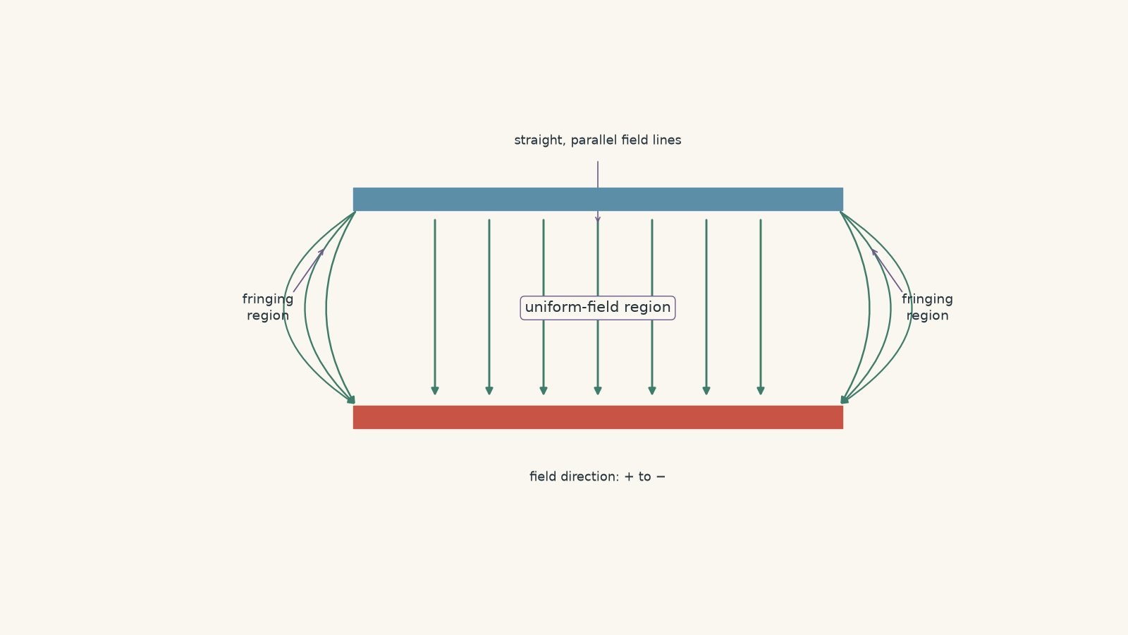
Near the edges:
- the field direction changes with position,
- the field magnitude can change with position,
- \(E=V/d\) no longer gives the exact local field.
The equation can still describe the characteristic or average field scale, but it should not be treated as the exact field at every point.
Here is the key distinction:
A known potential difference across a known distance does not, by itself, prove that the electric field is uniform.
The geometry and surrounding charge distribution matter too.
Does making the plates larger increase \(E\)?
Suppose the voltage and separation stay fixed, but each plate is made wider.
A student might predict a larger field because there is “more charged metal”.
For an ideal parallel-plate field maintained at a fixed potential difference, however,
\[
E=\frac{V}{d}
\]
does not contain plate area.
Making the plates larger mainly makes the central uniform-field approximation valid over a larger region. It does not automatically increase the ideal central field when \(V\) and \(d\) are unchanged.
This is one reason you should not treat equations as lists of variables and assume that every physical change must appear somewhere in the formula. Some changes affect whether the model is valid rather than the numerical value predicted by the model.
08Voltage is not the same thing as electric field
Another tempting misconception is that a point with a high voltage must have a strong electric field.
Not necessarily.
Electric field depends on how rapidly the potential changes with position.
Imagine a whole conducting plate at \(1000\ \text{V}\). Every point on that conductor can have the same potential, so there is no potential change as you move along its surface. The tangential electric field there is zero even though the potential itself is \(1000\ \text{V}\).
What matters is the gradient of potential, not simply whether the numerical value of the potential is large.
This is similar to altitude. Standing on a high but perfectly flat plateau means you are high above sea level, but you are not standing on a steep slope.
Again, the analogy has limits, but it captures the distinction between potential and potential gradient nicely.
09Questions and solutions
Question 1
Two parallel plates are separated by \(3.0\ \text{mm}\). The left plate is at \(+12\ \text{V}\), and the right plate is at \(0\ \text{V}\).
Calculate the electric field strength between the plates and state its direction.
Solution 1
The field strength is \(4.0\times10^3\ \text{V m}^{-1}\), directed from the left plate towards the right plate.
The field is approximately uniform, so
\[
E=\frac{V}{d}.
\]
Convert the separation:
\[
d=3.0\ \text{mm}=3.0\times10^{-3}\ \text{m}.
\]
The potential difference is \(12\ \text{V}\), giving
\[
\begin{aligned}
E&=\frac{12}{3.0\times10^{-3}}\\
&=4.0\times10^3\ \text{V m}^{-1}.
\end{aligned}
\]
The electric field points from higher potential to lower potential, so it points from the \(+12\ \text{V}\) left plate towards the \(0\ \text{V}\) right plate.
A common mistake is to give only \(4000\) with no unit or direction. Electric field is a vector quantity, so both matter.
Question 2
Two large horizontal plates are \(20\ \text{mm}\) apart and maintained at a potential difference of \(800\ \text{V}\). An electron starts from rest halfway between them.
Assume the field is uniform and ignore gravity.
The electron mass is \(9.11\times10^{-31}\ \text{kg}\), and the magnitude of its charge is \(1.60\times10^{-19}\ \text{C}\).
Calculate:
a. the electric field strength,
b. the magnitude of the electron’s acceleration,
c. the time taken for the electron to reach the positive plate.
Solution 2
The electric field is \(4.0\times10^4\ \text{V m}^{-1}\), the electron’s acceleration magnitude is approximately \(7.0\times10^{15}\ \text{m s}^{-2}\), and it reaches the positive plate after about \(1.7\times10^{-9}\ \text{s}\).
First, convert the plate separation:
\[
d=20\ \text{mm}=2.0\times10^{-2}\ \text{m}.
\]
For part a,
\[
\begin{aligned}
E&=\frac{V}{d}\\
&=\frac{800}{2.0\times10^{-2}}\\
&=4.0\times10^4\ \text{V m}^{-1}.
\end{aligned}
\]
For part b, the electric force magnitude is
\[
\begin{aligned}
F&=qE\\
&=(1.60\times10^{-19})(4.0\times10^4)\\
&=6.4\times10^{-15}\ \text{N}.
\end{aligned}
\]
Then, using \(F=ma\),
\[
\begin{aligned}
a&=\frac{F}{m}\\
&=\frac{6.4\times10^{-15}}{9.11\times10^{-31}}\\
&\approx7.0\times10^{15}\ \text{m s}^{-2}.
\end{aligned}
\]
The electron is halfway between the plates, so it travels
\[
s=10\ \text{mm}=1.0\times10^{-2}\ \text{m}.
\]
It starts from rest. For constant acceleration,
\[
s=ut+\frac12at^2.
\]
Since \(u=0\),
\[
t=\sqrt{\frac{2s}{a}}.
\]
Therefore,
\[
\begin{aligned}
t
&=\sqrt{\frac{2(1.0\times10^{-2})}{7.0\times10^{15}}}\\
&\approx1.7\times10^{-9}\ \text{s}.
\end{aligned}
\]
The tempting mistake is to make the electron accelerate in the electric-field direction. Its charge is negative, so its force and acceleration are opposite the field, towards the positive plate.
Question 3
Capacitor A has parallel plates separated by \(4.0\ \text{mm}\) with a potential difference of \(240\ \text{V}\).
Capacitor B has plates separated by \(15\ \text{mm}\) with a potential difference of \(750\ \text{V}\).
A proton is placed in the central region of each capacitor.
a. Which capacitor produces the larger electric force on the proton?
b. A student says, “It must be B because 750 V is much larger than 240 V.” Explain precisely what is wrong with this reasoning.
c. If the plates of capacitor A are made three times wider while its voltage and separation remain fixed, what happens to the ideal central field?
Solution 3
Capacitor A produces the larger force. The student’s reasoning fails because electric field depends on potential difference per unit separation, not potential difference alone, and making A’s plates wider does not change its ideal central field when \(V\) and \(d\) remain fixed.
For capacitor A,
\[
\begin{aligned}
E_A&=\frac{240}{4.0\times10^{-3}}\\
&=6.0\times10^4\ \text{V m}^{-1}.
\end{aligned}
\]
For capacitor B,
\[
\begin{aligned}
E_B&=\frac{750}{15\times10^{-3}}\\
&=5.0\times10^4\ \text{V m}^{-1}.
\end{aligned}
\]
Therefore,
\[
E_A>E_B.
\]
Since the same proton is placed in each field and
\[
F=qE,
\]
the larger electric field produces the larger force. Thus,
\[
F_A>F_B.
\]
The tempting route is to compare \(750\ \text{V}\) directly with \(240\ \text{V}\). But voltage is not field strength. Capacitor B spreads its larger potential difference across a much larger gap.
For part c,
\[
E_A=\frac{V}{d}
\]
is unchanged because neither \(V\) nor \(d\) changes.
The wider plates can improve the uniform-field approximation by moving edge effects farther from the central region. Plate area affects the geometry of the approximation, but it does not appear in \(E=V/d\) for an ideal field maintained at fixed \(V\) and \(d\).
Question 4
A proton enters horizontally midway between two parallel plates with speed \(3.0\times10^6\ \text{m s}^{-1}\). The plates are \(40\ \text{mm}\) long, \(12\ \text{mm}\) apart, and have a potential difference of \(600\ \text{V}\).
Assume the field is uniform inside the plate region and zero immediately after the proton leaves it. Ignore gravity.
A second apparatus is built with plates twice as long and twice as far apart. The voltage is also doubled. The proton enters the second apparatus with the same horizontal speed.
Without doing more calculation than necessary, compare:
a. the electric field strengths,
b. the proton’s vertical acceleration,
c. the time each proton spends between the plates,
d. the vertical velocity of each proton as it leaves the plates,
e. the vertical deflection accumulated while each proton is between the plates.
Solution 4
The two apparatuses have the same electric field and the same vertical acceleration, but the proton spends twice as long in the second field, leaves with twice the vertical velocity, and accumulates four times the vertical deflection while between the plates.
For the first apparatus,
\[
E_1=\frac{V}{d}.
\]
For the second apparatus, both \(V\) and \(d\) double:
\[
E_2=\frac{2V}{2d}=\frac{V}{d}=E_1.
\]
So the fields are equal.
Since
\[
F=qE
\]
and
\[
a=\frac{F}{m}=\frac{qE}{m},
\]
the same proton experiences the same vertical acceleration in both apparatuses.
Now consider the time spent between the plates. The electric force is vertical, so under the stated model it does not alter the proton’s horizontal velocity. The second plates are twice as long, so
\[
t_2=2t_1.
\]
The vertical exit speed follows from
\[
v_y=u_y+a_yt.
\]
The proton enters horizontally, so \(u_y=0\). Therefore,
\[
v_y=a_yt.
\]
Because the acceleration is unchanged but the time doubles,
\[
v_{y,2}=2v_{y,1}.
\]
Finally, the vertical displacement inside the field is
\[
y=u_yt+\frac12a_yt^2.
\]
Again \(u_y=0\), so
\[
y=\frac12a_yt^2.
\]
Doubling the time therefore gives
\[
y_2=\frac12a_y(2t_1)^2=4y_1.
\]
The tempting prediction is that “doubling everything should leave everything unchanged”, because \(E=V/d\) remains constant. That only fixes the field and therefore the acceleration. The plate length controls how long the acceleration acts. A constant acceleration acting for twice as long produces twice the velocity change and four times the displacement.
This is an important modelling habit: preserving one quantity does not preserve every outcome that depends on it.
Question 5
Two large plates are \(30\ \text{mm}\) apart with a total potential difference of \(600\ \text{V}\).
Student A immediately calculates
\[
E=\frac{600}{0.030}=2.0\times10^4\ \text{V m}^{-1}
\]
and claims that this must be the electric field at every point between the plates.
A probe is then used along a straight line from the high-potential plate to the low-potential plate. Over three consecutive \(10\ \text{mm}\) regions, the measured potential drops are:
- first region: \(120\ \text{V}\),
- second region: \(180\ \text{V}\),
- third region: \(300\ \text{V}\).
Assume the potential changes linearly within each of those three regions.
a. Determine the electric field magnitude in each region.
b. Explain why Student A’s calculation still gives \(2.0\times10^4\ \text{V m}^{-1}\), despite none of the three regions having that field strength.
c. A proton travels from the high-potential plate to the low-potential plate. Compare the total electrical work done on it with the work that would have been done in a genuinely uniform \(2.0\times10^4\ \text{V m}^{-1}\) field across the same \(30\ \text{mm}\).
d. What does this example reveal about the real limitation of \(E=V/d\)?
Solution 5
The three field magnitudes are \(1.2\times10^4\), \(1.8\times10^4\), and \(3.0\times10^4\ \text{V m}^{-1}\). Student A has calculated the average potential gradient across the whole gap, not the local field in each region. Despite the different local fields, the proton receives the same total electrical work as it would in a uniform field with the same total potential difference.
Each region has width
\[
10\ \text{mm}=1.0\times10^{-2}\ \text{m}.
\]
For the first region,
\[
\begin{aligned}
E_1&=\frac{120}{1.0\times10^{-2}}\\
&=1.2\times10^4\ \text{V m}^{-1}.
\end{aligned}
\]
For the second,
\[
\begin{aligned}
E_2&=\frac{180}{1.0\times10^{-2}}\\
&=1.8\times10^4\ \text{V m}^{-1}.
\end{aligned}
\]
For the third,
\[
\begin{aligned}
E_3&=\frac{300}{1.0\times10^{-2}}\\
&=3.0\times10^4\ \text{V m}^{-1}.
\end{aligned}
\]
So the field becomes stronger as the proton moves across the gap.
Student A used the total voltage drop divided by the total distance:
\[
\frac{600}{0.030}=2.0\times10^4\ \text{V m}^{-1}.
\]
That value is the average potential drop per metre over the whole \(30\ \text{mm}\).
We can check this from the three regions. Each region has the same width, so the average field magnitude is
\[
\begin{aligned}
E_{\text{avg}}
&=\frac{E_1+E_2+E_3}{3}\\
&=\frac{1.2+1.8+3.0}{3}\times10^4\\
&=2.0\times10^4\ \text{V m}^{-1}.
\end{aligned}
\]
The calculation was therefore not numerically meaningless. The mistake was interpreting an average field as the local field everywhere.
For part c, the total work done by the electric field on a proton moving through a potential drop \(V\) depends on the proton’s charge and the total potential difference:
\[
W=qV.
\]
Using
\[
q=1.60\times10^{-19}\ \text{C}
\]
and
\[
V=600\ \text{V},
\]
\[
\begin{aligned}
W
&=(1.60\times10^{-19})(600)\\
&=9.6\times10^{-17}\ \text{J}.
\end{aligned}
\]
A genuinely uniform \(2.0\times10^4\ \text{V m}^{-1}\) field across \(0.030\ \text{m}\) would have
\[
V=Ed=(2.0\times10^4)(0.030)=600\ \text{V}.
\]
So it would do exactly the same total work:
\[
W=9.6\times10^{-17}\ \text{J}.
\]
This is the hinge in the problem. The proton can gain the same total kinetic energy even though its acceleration history is different.
In the non-uniform field, the proton’s electric force becomes larger as it crosses the three regions because
\[
F=qE.
\]
In the uniform field, the force remains constant. Yet both paths involve the same overall 600 V decrease in potential.
The tempting argument is, “Same \(V\) and same \(d\), therefore same field everywhere.” What actually follows is only that the overall potential change per total distance is \(V/d\). To identify that value with the local electric field at every point, you need the additional physical assumption that the field is uniform.
That is the real limit of
\[
E=\frac{V}{d}.
\]
It is powerful because an ideal parallel-plate geometry makes the field nearly uniform in the central region. It is not the definition of electric field for every possible arrangement.
Once that distinction is clear, the next useful step is to connect electric fields to the motion and energy of charged particles. The field tells you the force through \(F=qE\), while the potential difference tells you the energy transfer through \(W=qV\). Those two descriptions are closely related, but they answer different questions: one tells you what happens to the particle’s motion at a particular place, and the other tells you how much energy changes across a journey.