
The Exponential Radioactive Decay Law: HSC Physics Guide
Learn how radioactive nuclei decrease exponentially using N = N₀ exp(-λt), with clear explanations, worked examples, and challenging HSC-style questions.
Suppose a radioactive sample starts with 1,000,000 unstable nuclei. If 10% of the nuclei decay in the first minute, should another 10% of the original 1,000,000 decay in the second minute?
No. If 10% decay each minute, the second 10% is taken from the nuclei still there. So the sample goes \(1,000,000 \rightarrow 900,000 \rightarrow 810,000 \rightarrow 729,000\).
The number lost each minute gets smaller, even though the fraction lost stays the same. That simple idea is the reason radioactive decay follows an exponential law rather than a straight line.
The same fraction decays each interval
- Start
N = 1000
Initial population: 1000 nuclei
- After 1 interval
1000 → 900
10% of 1000 = 100 decay
900 nuclei remain
- After 2 intervals
900 → 810
10% of 900 = 90 decay
810 nuclei remain
- After 3 intervals
810 → 729
10% of 810 = 81 decay
729 nuclei remain
01The physical idea behind radioactive decay
A radioactive nucleus has a probability of decaying, but we cannot predict exactly when one particular nucleus will decay.
For a large collection of identical unstable nuclei, however, the overall behaviour is predictable. At any moment, each nucleus has the same characteristic tendency to decay. If there are twice as many nuclei present, there are twice as many opportunities for decay.
This means the decay rate is proportional to the number of nuclei remaining:
\[ -\frac{dN}{dt}=\lambda N \]
Here:
- \(N\) is the number of undecayed nuclei at time \(t\),
- \(t\) is the elapsed time,
- \(\lambda\) is the decay constant,
- \(\lambda\) has units of inverse time, such as \(\mathrm{s^{-1}}\) or \(\mathrm{h^{-1}}\).
The minus sign appears because \(N\) decreases as time increases.
The important physical point is that \(\lambda\) is constant for a particular radioactive isotope under the conditions being considered, but the number of nuclei available to decay is not constant.
So the decay rate gets smaller as the sample gets smaller.
02The exponential decay law
Solving that relationship gives the HSC radioactive decay law:
\[ N=N_0\exp(-\lambda t) \]
where \(N_0\) is the number of undecayed nuclei at \(t=0\).
You can also write
\[ N=N_0e^{-\lambda t} \]
because \(\exp(x)\) means \(e^x\), where \(e\approx2.718\).
The factor
\[ \exp(-\lambda t) \]
tells you what fraction of the original sample remains.
So:
\[ \frac{N}{N_0}=\exp(-\lambda t) \]
This is often the easiest way to think about the equation. The formula is not saying that a fixed number of nuclei disappears every second. It is saying that the fraction remaining depends exponentially on time.
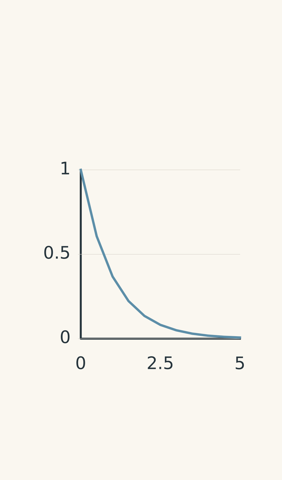
- N/N₀ = exp(−λt), λ = 1 s⁻¹
A useful check: the exponent must have no units
The quantity \(\lambda t\) appears in an exponent, so it must be dimensionless.
That means your units for \(\lambda\) and \(t\) must match.
For example:
- \(\lambda\) in \(\mathrm{s^{-1}}\) requires \(t\) in seconds.
- \(\lambda\) in \(\mathrm{h^{-1}}\) requires \(t\) in hours.
A very common HSC error is putting \(t=5\) into the equation when \(t\) is 5 minutes but \(\lambda\) is given in \(\mathrm{s^{-1}}\).
Convert first.
03What the decay constant actually means
A large \(\lambda\) means the sample decays quickly.
A small \(\lambda\) means it decays slowly.
But don’t interpret \(\lambda\) as “the exact percentage that disappears every second”. More precisely, it describes the characteristic rate of decay of the current population.
For a very short time interval, the fraction that decays is approximately \(\lambda\Delta t\). Over a substantial time interval, you must use the exponential law.
That’s why this tempting calculation is wrong:
\[ N=N_0(1-\lambda t) \]
It treats the loss as linear. Radioactive decay is not linear.
For example, if \(\lambda=0.002\ \mathrm{s^{-1}}\), it is tempting to say that 0.2% of the original sample disappears every second. But after 1000 s, that would predict zero nuclei:
\[ 1-\lambda t=1-(0.002)(1000)=0 \]
The exponential law instead gives
\[ \frac{N}{N_0}=e^{-2}\approx0.135 \]
so about 13.5% remains.
The difference comes from one crucial fact: after each small time interval, there are fewer nuclei available to decay.
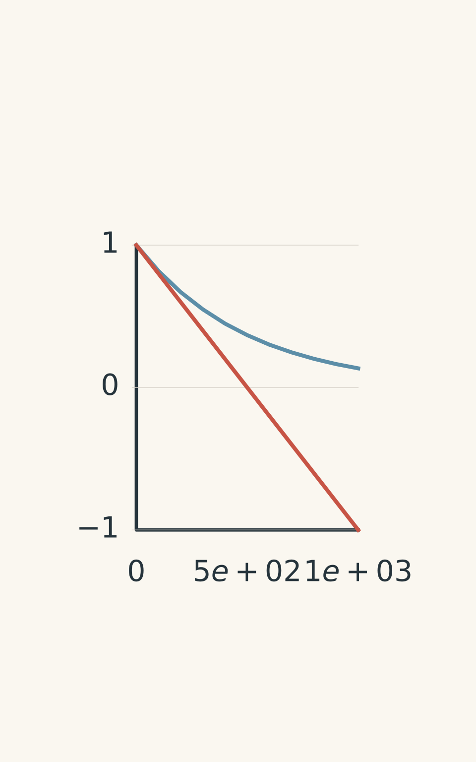
- Exponential: exp(−λt)
- Linear: 1 − λt
04Half-life is built into the exponential law
A half-life is simply the time required for the number of undecayed nuclei to fall to half its current value.
Set \(N=N_0/2\) in the decay law:
\[ \frac{N_0}{2} = N_0\exp(-\lambda T_{1/2}) \]
Cancel \(N_0\):
\[ \frac12=\exp(-\lambda T_{1/2}) \]
Taking the natural logarithm gives:
\[ T_{1/2}=\frac{\ln 2}{\lambda} \]
where \(T_{1/2}\) is the half-life and \(\ln\) is the natural logarithm.
This gives the familiar pattern:
- after 1 half-life: \(N=N_0/2\),
- after 2 half-lives: \(N=N_0/4\),
- after 3 half-lives: \(N=N_0/8\),
- after 4 half-lives: \(N=N_0/16\).
Notice what is happening. The same fraction remains after each half-life, not the same number of nuclei.
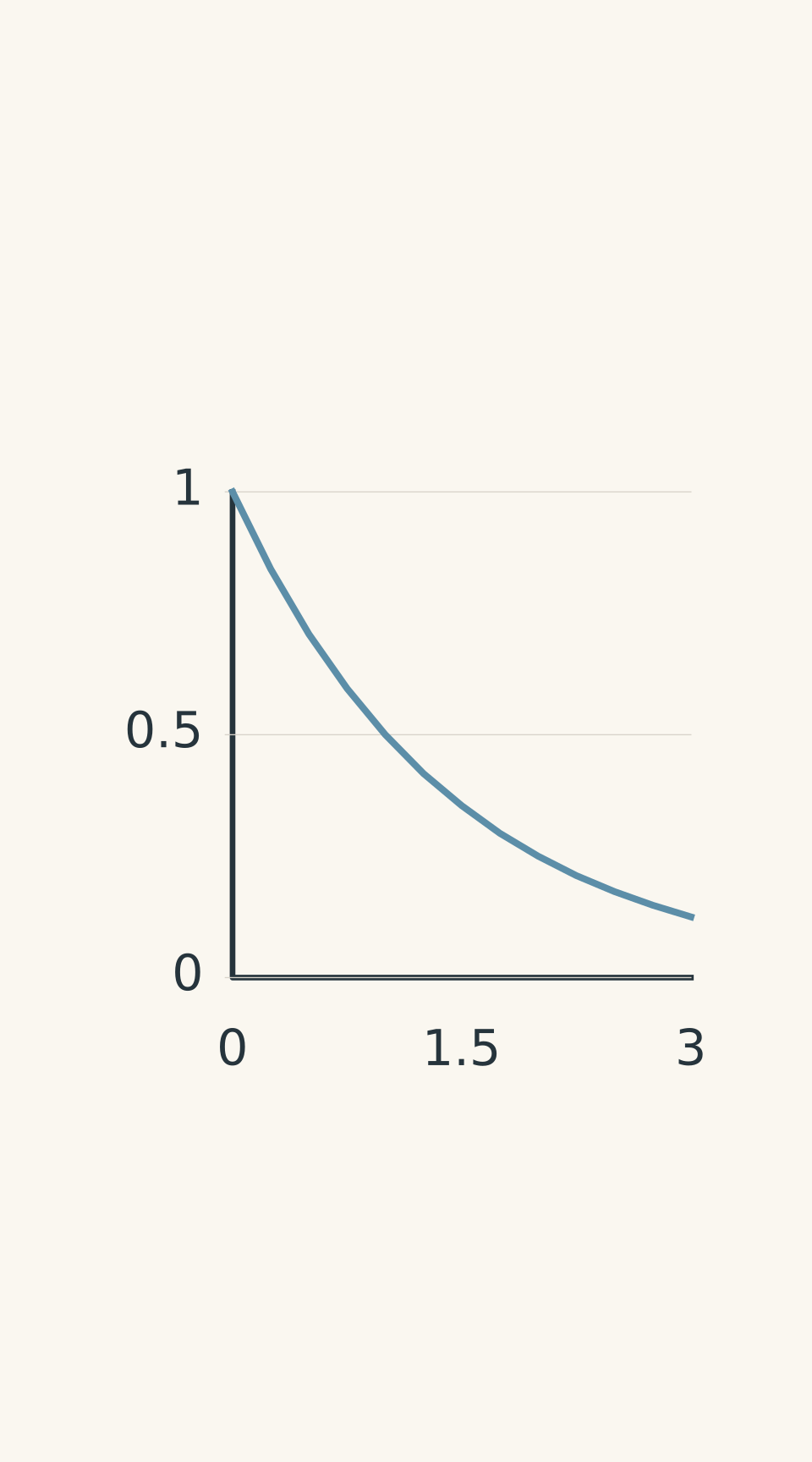
- Exponential decay
The relationship between \(\lambda\) and half-life is covered in more detail in Decay constant and half-life: HSC Physics explained.
05A powerful rearrangement for two measurements
You will often be given the number of nuclei at two different times rather than \(N_0\).
Suppose:
\[ N_1=N_0e^{-\lambda t_1} \]
and
\[ N_2=N_0e^{-\lambda t_2} \]
Divide the equations:
\[ \frac{N_2}{N_1} = e^{-\lambda(t_2-t_1)} \]
This is useful because \(N_0\) disappears.
You can then find the decay constant with:
\[ \lambda = \frac{1}{t_2-t_1} \ln\left(\frac{N_1}{N_2}\right) \]
Or, if \(\lambda\) is already known, you can find the elapsed time:
\[ t_2-t_1 = \frac{1}{\lambda} \ln\left(\frac{N_1}{N_2}\right) \]
This method is especially useful when the question gives a measurement at some non-zero time and asks what happens later.
06Worked example: finding the number of nuclei remaining
A radioactive sample initially contains \(1.50\times10^{15}\) nuclei. Its decay constant is \(4.00\times10^{-4}\ \mathrm{s^{-1}}\). How many nuclei remain after \(1800\ \mathrm{s}\)?
Step 1
\[ N=N_0\exp(-\lambda t) \]
Step 2
\[ N = (1.50\times10^{15}) \exp[-(4.00\times10^{-4})(1800)] \]
Step 3
\[ \lambda t=(4.00\times10^{-4})(1800)=0.720 \]
So:
\[ N=(1.50\times10^{15})e^{-0.720} \]
Step 4
\[ N=7.30\times10^{14}\ \text{nuclei} \]
Step 5
About \(7.30\times10^{14}\) nuclei remain, which is about 48.7% of the original sample. The other 51.3% have decayed.
The result is less than \(N_0\), as it must be. If your calculation gives a number larger than \(N_0\), check the sign in the exponent.
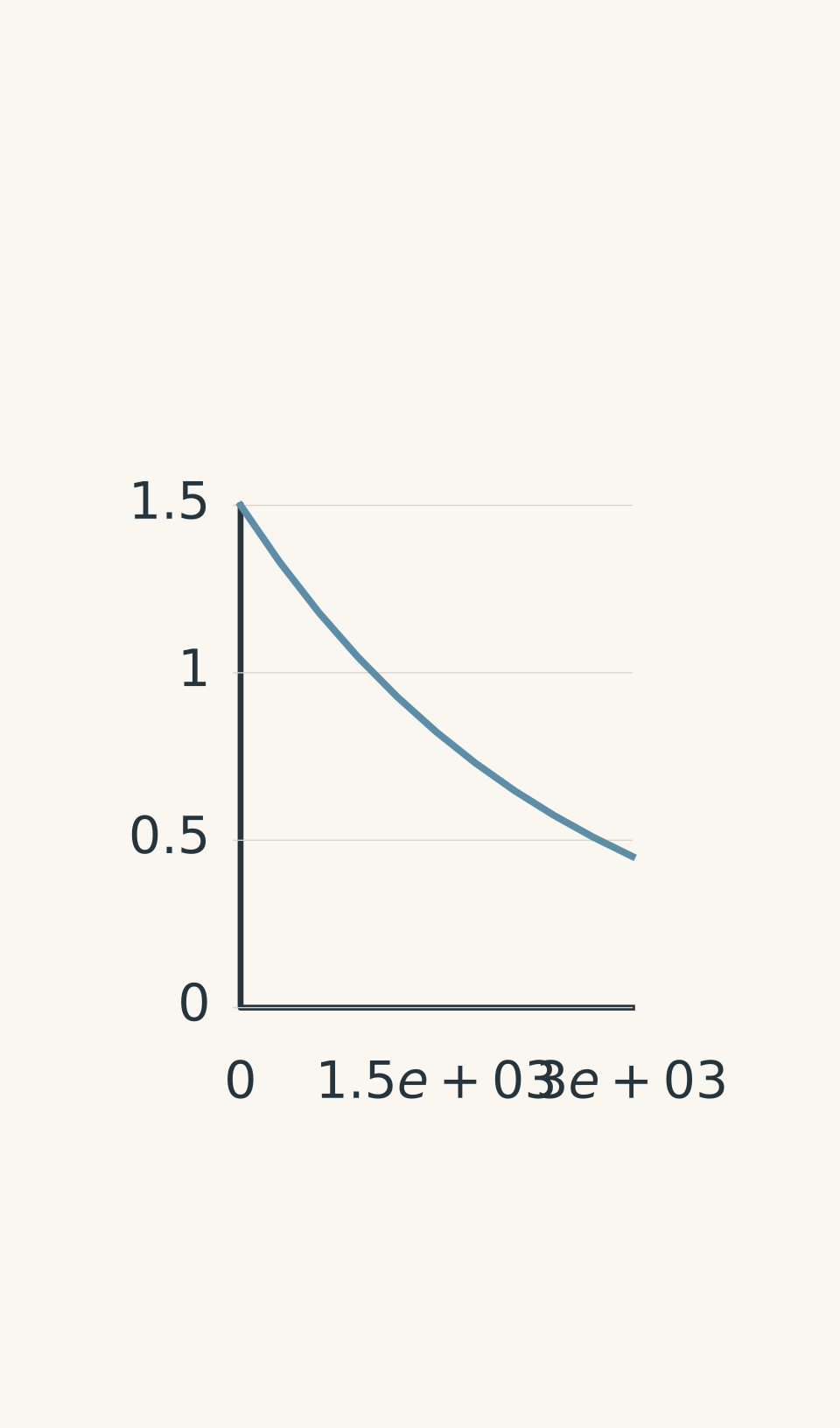
- N(t): nuclei remaining
07Worked example: finding the decay constant from measurements
A sample initially contains \(4.80\times10^{14}\) nuclei. After \(2.50\ \mathrm{h}\), \(3.00\times10^{14}\) nuclei remain.
Find:
- the decay constant in \(\mathrm{s^{-1}}\),
- the half-life,
- the number of nuclei remaining after \(7.00\ \mathrm{h}\).
Step 1
\[ N=N_0\exp(-\lambda t) \]
For the first measurement:
\[ 3.00\times10^{14} = (4.80\times10^{14}) e^{-\lambda(2.50)} \]
Here, time is in hours, so temporarily find \(\lambda\) in \(\mathrm{h^{-1}}\).
Step 2
\[ \frac{3.00}{4.80}=e^{-2.50\lambda} \]
Step 3
\[ \ln\left(\frac{3.00}{4.80}\right) = -2.50\lambda \]
Therefore:
\[ \lambda = \frac{1}{2.50} \ln\left(\frac{4.80}{3.00}\right) \]
\[ \lambda=0.188\ \mathrm{h^{-1}} \]
Step 4
Since \(1\ \mathrm{h}=3600\ \mathrm{s}\):
\[ \lambda = \frac{0.188}{3600} = 5.22\times10^{-5}\ \mathrm{s^{-1}} \]
Step 5
\[ T_{1/2} = \frac{\ln2}{\lambda} = \frac{0.693}{0.188} \]
\[ T_{1/2}=3.69\ \mathrm{h} \]
Step 6
Use the original \(N_0\):
\[ N = (4.80\times10^{14}) e^{-(0.188)(7.00)} \]
\[ N=1.29\times10^{14}\ \text{nuclei} \]
So about \(1.29\times10^{14}\) nuclei remain after \(7.00\ \mathrm{h}\).
The tempting shortcut here is to calculate \((N_0-N)/t\) and call that \(\lambda\). That gives an average loss per unit time, not the exponential decay constant. The decay rate changes as \(N\) changes.
08What if the detector measures counts instead of nuclei?
In an experiment, you usually cannot count the nuclei directly. A detector records radiation events.
If the detector efficiency stays constant and there is no background count, the measured count rate is proportional to the number of radioactive nuclei remaining. Therefore the count rate follows the same exponential factor:
\[ C=C_0\exp(-\lambda t) \]
where \(C\) is the measured count rate and \(C_0\) is the initial count rate.
This is a useful extension of the same law, not a different decay process.
The catch is background radiation. If the detector records a constant background \(B\), then the measured count rate is better represented by:
\[ C=C_0\exp(-\lambda t)+B \]
The exponential law applies to the radioactive part of the signal, not automatically to everything the detector records.
Detector signal = decay + background
| Source → detector | Radioactive source → detector The detector records radiation from the source. |
|---|---|
| Signal separation | C(t) = C₀ exp(−λt) + B Radioactive signal decays; background B stays constant. |
09The traps worth remembering
| Tempting prediction | What the decay law actually says |
|---|---|
| A constant \(\lambda\) means a constant number decay each second. | The fractional decay behaviour is constant; the absolute number decaying falls as \(N\) falls. |
| Subtract the same number after every equal time interval. | Multiply by the same survival fraction after every equal time interval. |
| \(\lambda\) can be used with any time unit. | \(\lambda\) and \(t\) must use matching units. |
| Count rate always equals the number of radioactive nuclei. | Count rate is a measured signal proportional to the radioactive population only under suitable detector assumptions. |
| \(N_0\) means the number of nuclei ever produced. | \(N_0\) is the number present at the chosen \(t=0\). |
| The exponential curve reaches zero after a fixed time. | The ideal exponential approaches zero; an actual finite sample eventually has individual decay events and can reach zero nuclei. |
10Questions and solutions
Question 1
A radioactive isotope has \(N_0=7.0\times10^{12}\) undecayed nuclei and a decay constant of \(1.5\times10^{-3}\ \mathrm{s^{-1}}\).
How many nuclei remain after \(500\ \mathrm{s}\)?
Solution 1
\(\mathbf{3.31\times10^{12}}\) nuclei remain.
Step 1: Use the decay law.
\[ N=N_0\exp(-\lambda t) \]
Step 2: Substitute the values.
\[ N = (7.0\times10^{12}) \exp[-(1.5\times10^{-3})(500)] \]
Step 3: Calculate the exponent.
\[ \lambda t=0.750 \]
Therefore:
\[ N=(7.0\times10^{12})e^{-0.750} \]
\[ N=3.31\times10^{12}\ \text{nuclei} \]
About 47.2% remains. The result is smaller than the initial number, and the decrease is exponential rather than linear.
Question 2
A radioactive sample contains \(9.0\times10^{16}\) nuclei initially. After \(3.0\ \mathrm{h}\), \(5.0\times10^{16}\) nuclei remain.
Find:
- the decay constant in \(\mathrm{s^{-1}}\),
- the half-life,
- the number of nuclei remaining after \(8.0\ \mathrm{h}\).
Solution 2
The decay constant is \(5.44\times10^{-5}\ \mathrm{s^{-1}}\), the half-life is \(3.54\ \mathrm{h}\), and \(1.88\times10^{16}\) nuclei remain after \(8.0\ \mathrm{h}\).
Step 1: Use the first measurement to find \(\lambda\).
\[ 5.0\times10^{16} = (9.0\times10^{16})e^{-3.0\lambda} \]
Divide by \(9.0\times10^{16}\):
\[ \frac{5.0}{9.0}=e^{-3.0\lambda} \]
Take \(\ln\):
\[ \lambda = \frac{1}{3.0} \ln\left(\frac{9.0}{5.0}\right) \]
\[ \lambda=0.196\ \mathrm{h^{-1}} \]
Convert to seconds:
\[ \lambda = \frac{0.196}{3600} = 5.44\times10^{-5}\ \mathrm{s^{-1}} \]
Step 2: Find the half-life.
\[ T_{1/2} = \frac{\ln2}{\lambda} = \frac{0.693}{0.196} \]
\[ T_{1/2}=3.54\ \mathrm{h} \]
Step 3: Calculate the population after \(8.0\ \mathrm{h}\).
\[ N = (9.0\times10^{16}) e^{-(0.196)(8.0)} \]
\[ N=1.88\times10^{16}\ \text{nuclei} \]
A tempting route is to assume that because \(4.0\times10^{16}\) nuclei disappeared in the first \(3.0\ \mathrm{h}\), another \(4.0\times10^{16}\) will disappear in the next \(3.0\ \mathrm{h}\). That would be a linear model. The exponential law instead applies the same fractional reduction to the nuclei currently present.
Question 3
A detector records \(960\) counts per minute from a radioactive source. Five minutes later it records \(360\) counts per minute.
Assume the detector efficiency is constant and there is no background radiation.
Find:
- the decay constant in \(\mathrm{min^{-1}}\),
- the time from the initial measurement until the count rate falls to \(100\) counts per minute.
Solution 3
The decay constant is \(0.196\ \mathrm{min^{-1}}\), and the count rate reaches \(100\) counts per minute about \(11.5\) minutes after the initial measurement.
Because the detector conditions are constant and there is no background, the count rate is proportional to the number of radioactive nuclei. It therefore has the same exponential dependence.
Step 1: Use the two measurements.
\[ \frac{C_2}{C_1} = e^{-\lambda\Delta t} \]
\[ \frac{360}{960} = e^{-5.0\lambda} \]
Step 2: Take the natural logarithm.
\[ \lambda = \frac{1}{5.0} \ln\left(\frac{960}{360}\right) \]
\[ \lambda=0.196\ \mathrm{min^{-1}} \]
Step 3: Find the time for the count rate to reach \(100\) counts per minute.
\[ 100 = 960e^{-0.196t} \]
So:
\[ t = \frac{1}{0.196} \ln\left(\frac{960}{100}\right) \]
\[ t=11.5\ \mathrm{min} \]
The important condition is the detector assumption. If there were a significant background count, applying the exponential law directly to the measured count rate would give the wrong \(\lambda\).
Question 4
An isotope has a decay constant of \(2.00\times10^{-3}\ \mathrm{s^{-1}}\) and initially contains \(1.00\times10^8\) nuclei.
A student argues:
“The decay constant is \(0.002\), so 0.2% of the original nuclei decay every second. After \(1000\) seconds, \(1000\times0.2\%=100\%\) will have decayed, so none will remain.”
Calculate the number of nuclei remaining after \(100\ \mathrm{s}\) and after \(1000\ \mathrm{s}\). Then explain precisely what is wrong with the student’s reasoning.
Solution 4
The sample has \(8.19\times10^7\) nuclei after \(100\ \mathrm{s}\) and \(3.68\times10^7\) nuclei after \(1000\ \mathrm{s}\). The student’s mistake is treating the decay as a fixed percentage of the original population each second rather than a decay process whose rate depends on the population currently remaining.
Step 1: Calculate the population after \(100\ \mathrm{s}\).
\[ N = (1.00\times10^8) e^{-(2.00\times10^{-3})(100)} \]
\[ N = (1.00\times10^8)e^{-0.200} \]
\[ N=8.19\times10^7\ \text{nuclei} \]
Step 2: Calculate the population after \(1000\ \mathrm{s}\).
\[ N = (1.00\times10^8) e^{-(2.00\times10^{-3})(1000)} \]
\[ N = (1.00\times10^8)e^{-2.00} \]
\[ N=3.68\times10^7\ \text{nuclei} \]
The tempting linear model is
\[ N=N_0(1-\lambda t) \]
but this is not the radioactive decay law. It can act as a rough approximation over a sufficiently tiny time interval, where \(\lambda\Delta t\) is very small.
The exact model says that the decay rate is proportional to the current number \(N\). As \(N\) falls, fewer nuclei are available to decay. So the absolute number lost per second falls too.
Question 5
A detector is monitoring a radioactive source. The detector has an unknown but constant background count rate.
The total measured count rates are:
| Time | Measured count rate |
|---|---|
| \(0\ \mathrm{h}\) | \(1000\) counts/min |
| \(4.0\ \mathrm{h}\) | \(600\) counts/min |
| \(8.0\ \mathrm{h}\) | \(400\) counts/min |
Assume:
- the radioactive part of the signal follows \(C=C_0\exp(-\lambda t)\),
- the background is constant,
- the detector efficiency does not change.
Determine:
- the background count rate,
- the decay constant in \(\mathrm{s^{-1}}\),
- the total count rate expected at \(16\ \mathrm{h}\).
Solution 5
The background is 200 counts/min, the decay constant is \(4.81\times10^{-5}\ \mathrm{s^{-1}}\), and the predicted total count rate at \(16\ \mathrm{h}\) is 250 counts/min.
The key is to separate the radioactive signal from the background before applying the exponential law.
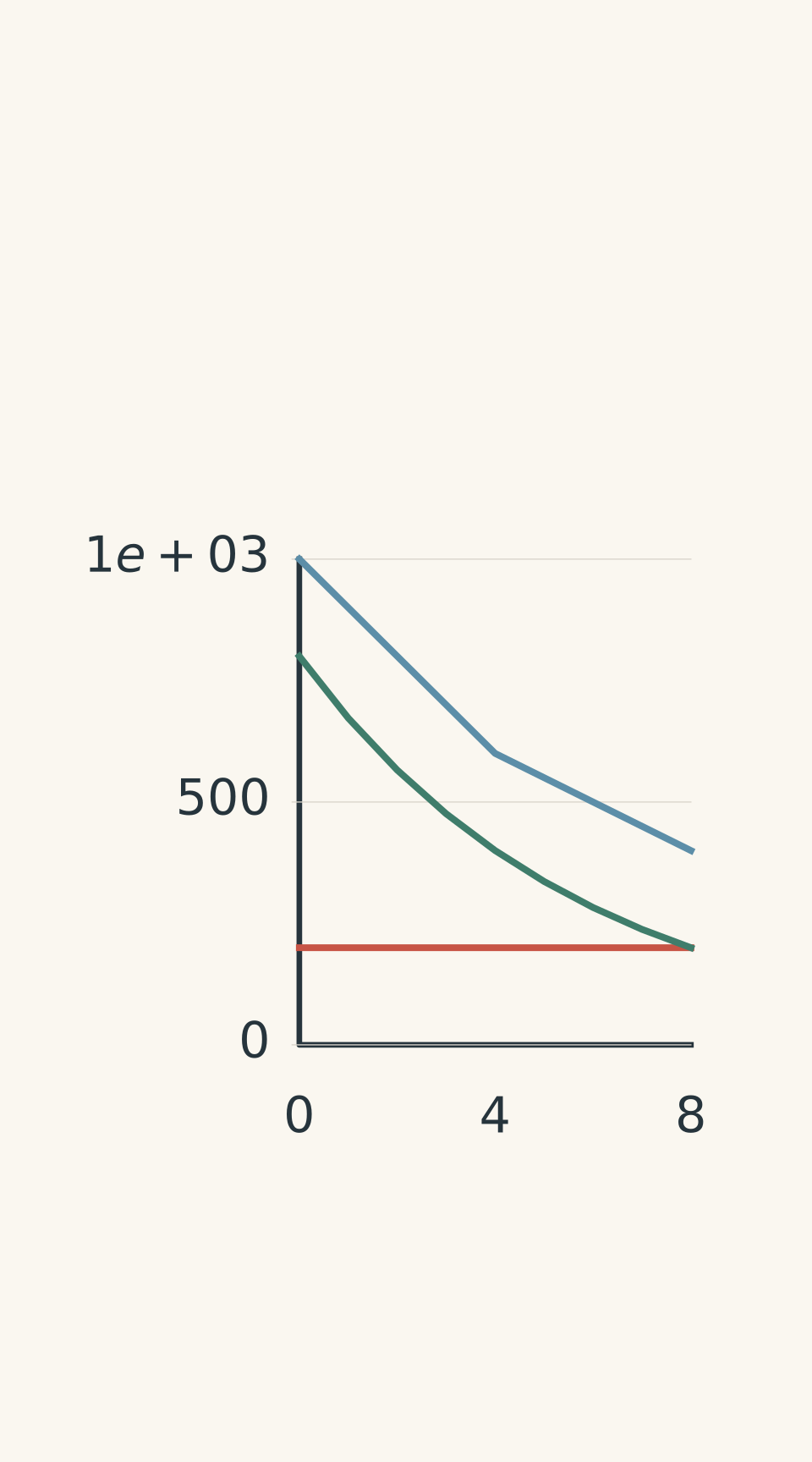
- Measured total
- Background = 200 counts/min
- Radioactive component (×½ per 4 h)
Step 1: Look at how the measured count rate changes.
From \(0\) to \(4\) hours, the count rate falls by:
\[ 1000-600=400\ \text{counts/min} \]
From \(4\) to \(8\) hours, it falls by:
\[ 600-400=200\ \text{counts/min} \]
The drops are not equal, so simply treating the measured values as \(N\) and using one exponential factor does not work.
But the radioactive part does lose the same fraction over each equal time interval.
Let the survival factor over \(4\) hours be \(r\).
The difference between successive measured values contains only the radioactive component, because the constant background cancels:
\[ \frac{600-400}{1000-600} = \frac{200}{400} = 0.5 \]
So the radioactive component is multiplied by \(0.5\) every \(4\) hours.
Step 2: Find the background.
Let the background be \(B\).
At \(t=0\), the radioactive component is:
\[ 1000-B \]
At \(t=4\ \mathrm{h}\), it is:
\[ 600-B \]
Since half the radioactive component remains after \(4\) hours:
\[ 600-B = 0.5(1000-B) \]
Expanding:
\[ 600-B=500-0.5B \]
Therefore:
\[ B=200\ \text{counts/min} \]
So the radioactive component initially contributes:
\[ 1000-200=800\ \text{counts/min} \]
Step 3: Find \(\lambda\).
After \(4\) hours, half of the radioactive component remains:
\[ e^{-4\lambda}=\frac12 \]
Therefore:
\[ 4\lambda=\ln2 \]
\[ \lambda=\frac{\ln2}{4} =0.173\ \mathrm{h^{-1}} \]
Convert to \(\mathrm{s^{-1}}\):
\[ \lambda = \frac{0.173}{3600} = 4.81\times10^{-5}\ \mathrm{s^{-1}} \]
Step 4: Predict the radioactive component at \(16\) hours.
Sixteen hours is four intervals of four hours.
The radioactive component therefore halves four times:
\[ 800 \rightarrow400 \rightarrow200 \rightarrow100 \rightarrow50 \]
So at \(16\) hours:
\[ C_{\text{radioactive}}=50\ \text{counts/min} \]
Add the constant background:
\[ C_{\text{total}}=50+200 \]
\[ \boxed{C_{\text{total}}=250\ \text{counts/min}} \]
The tempting route was to apply \(C=C_0e^{-\lambda t}\) directly to \(1000\), \(600\), and \(400\). That assumes the entire detector signal is radioactive. It cannot be correct here because a constant background does not decay.
This is a useful general lesson: the exponential law describes the radioactive component of a signal. Before using it on experimental data, check what else the detector is measuring.
The next useful step is being able to move confidently between \(\lambda\), half-life, remaining nuclei, and measured activity or count rate. Decay constant and half-life: HSC Physics explained develops that connection.