
Validating Projectile Motion Experimentally: HSC Physics
Learn how to design, analyse, and evaluate a practical test of projectile motion relationships using HSC Physics models, graphs, and experimental evidence.
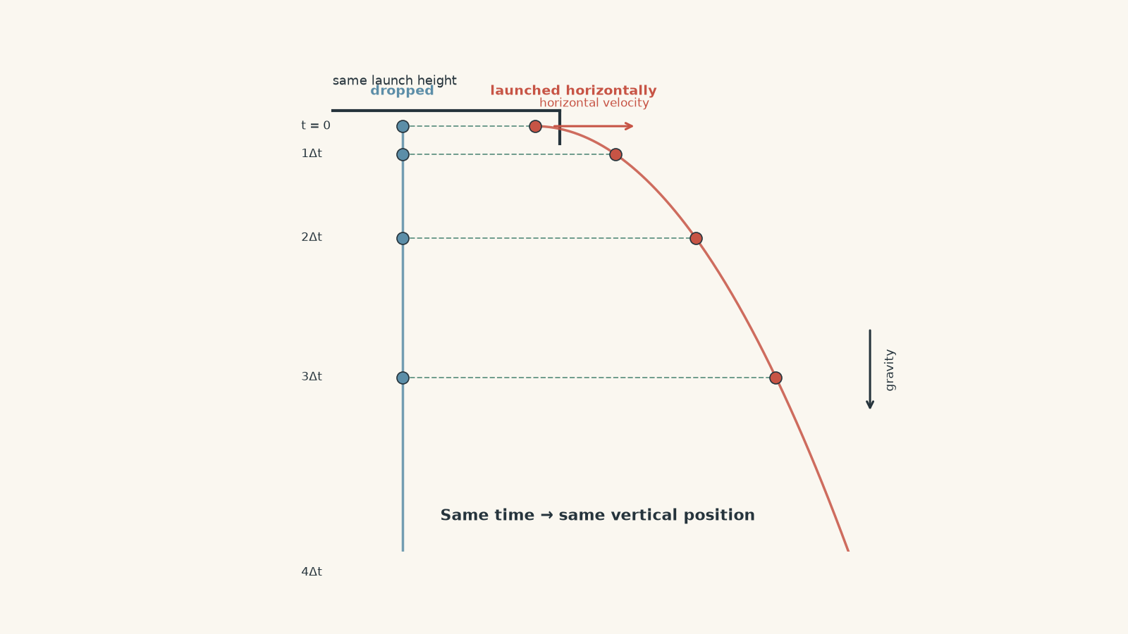
Drop one ball from a bench and fire an identical ball horizontally from the same height. Which one hits the floor first?
A common prediction is that the fired ball should stay up longer because it has “more motion”. Under the standard projectile model, though, they land at the same time. The horizontal speed changes how far the second ball travels, but not how quickly gravity pulls it down.
That is a neat prediction. It is also exactly the sort of claim physics should have to earn experimentally.
01What are we actually trying to validate?
For a projectile moving near Earth’s surface, the usual HSC model makes two important assumptions:
- gravitational acceleration is constant and vertically downward,
- air resistance is negligible.
Choose \(+x\) horizontally in the direction of launch and \(+y\) vertically upward. Then
\[ a_x = 0 \]
and
\[ a_y = -g \]
where \(g\) is the magnitude of gravitational acceleration, approximately \(9.8\ \text{m s}^{-2}\) near Earth’s surface.
That gives two motions happening at the same time:
\[ x = u_x t \]
and
\[ y = u_y t - \frac{1}{2}gt^2 \]
where:
- \(x\) is horizontal displacement in metres,
- \(y\) is vertical displacement in metres,
- \(u_x\) is the initial horizontal velocity in \(\text{m s}^{-1}\),
- \(u_y\) is the initial vertical velocity in \(\text{m s}^{-1}\),
- \(t\) is time in seconds.
For a horizontal launch, \(u_y=0\). The equations become
\[ x=u_x t \]
and
\[ y=-\frac{1}{2}gt^2 \]
The important idea is not merely that there are two equations. It is that the horizontal equation contains no vertical velocity, while the vertical equation contains no horizontal velocity.
You can picture the ball as having two separate dating lives. Horizontally, it keeps moving at the same rate. Vertically, gravity is the only serious relationship in its life. Both motions use the same clock, but they do not tell each other what to do.
That analogy has a limit. Once air resistance becomes important, the drag force depends on the projectile’s motion through the air. Horizontal and vertical behaviour can then become coupled.
02A prediction worth testing
Suppose a ball is fired horizontally from a height \(h\).
Its vertical displacement when it reaches the floor is \(y=-h\), so
\[ -h=-\frac{1}{2}gt^2 \]
which gives
\[ t=\sqrt{\frac{2h}{g}} \]
Notice what is missing: \(u_x\).
The model therefore predicts that the flight time does not depend on horizontal launch speed.
The horizontal range \(R\) is
\[ R=u_x t \]
so
\[ R=u_x\sqrt{\frac{2h}{g}} \]
At a fixed launch height, the model predicts
\[ R\propto u_x \]
Double the horizontal launch speed and the range should double.
At a fixed horizontal speed,
\[ R^2=\frac{2u_x^2}{g}h \]
so
\[ R^2\propto h \]
These give us several experimental tests rather than one vague question about whether the path “looks parabolic”.
| Model prediction | Useful experimental test |
|---|---|
| \(a_x=0\) | Plot horizontal position \(x\) against time \(t\). It should be linear. |
| \(a_y=-g\) | Plot downward displacement against \(t^2\). It should be linear. |
| \(R\propto u_x\) at fixed \(h\) | Plot \(R\) against measured \(u_x\). |
| \(R^2\propto h\) at fixed \(u_x\) | Plot \(R^2\) against \(h\). |
| \(t\) is independent of \(u_x\) | Change \(u_x\) while keeping \(h\) constant and compare flight times. |
That is what “validating projectile relationships” should mean. You test specific predictions of the model.
03First design: roll a ball off a bench
The simplest version needs very little equipment.
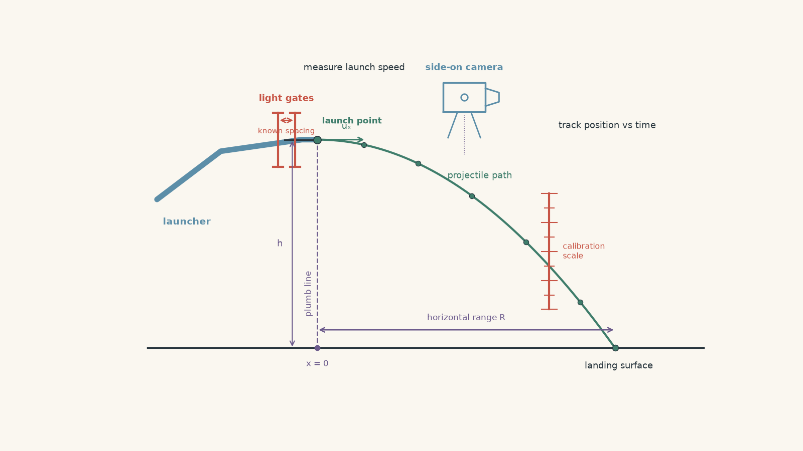
Place a ramp on a bench so that its final section is horizontal. A ball rolls down the ramp, travels along the horizontal section, and leaves the edge of the bench.
Directly below the launch point, hang a plumb line to mark the horizontal origin on the floor. Further out, place paper over carbon paper or another impact-marking surface so the first point of contact can be located.
Measure:
- the vertical drop \(h\),
- the horizontal range \(R\),
- the release position on the ramp.
Repeat each release several times.
What should happen?
Before looking at any measurements, predict the trend.
If the ball is released from higher up the ramp, it should leave faster. If the launch height above the floor stays unchanged, its time in the air should stay approximately unchanged. The extra speed should therefore appear mainly as extra horizontal range.
So a higher release point should produce a larger \(R\).
That is evidence in the right direction, but there is a problem.
The first design does not measure launch speed
A release position on a ramp is not the quantity in the projectile equation. The equation contains \(u_x\).
You might try to calculate the launch speed from gravitational potential energy. But now you need to account for the ball’s rotational kinetic energy, rolling behaviour, friction, and any losses in the ramp.
The experiment has accidentally mixed two models:
- the mechanics of a ball travelling down the ramp,
- the projectile motion after the ball leaves it.
If your purpose is to validate \(R\propto u_x\), measuring \(u_x\) directly is much cleaner.
04Revised design: measure the variables the equation actually contains
A stronger setup measures the projectile’s launch velocity and trajectory directly.
From left to right, arrange:
- a launcher or ramp with a short horizontal exit section,
- a pair of light gates close to the exit, separated by a known horizontal distance,
- the launch edge,
- the projectile’s flight region,
- an impact surface or catch box.
Place a camera side-on to the motion. Its optical axis should be as close as possible to perpendicular to the plane of the projectile’s path. Put a calibration scale in the same plane as the motion.
The ball passes the first light gate and then the second. If their separation is \(d\) and the travel time between them is \(\Delta t\), its horizontal launch speed is approximately
\[ u_x=\frac{d}{\Delta t} \]
The ball then leaves the launcher, crosses the camera’s field of view, and lands on the impact surface. The video provides position at known times, while the impact mark provides an independent measurement of total range.
This setup can test much more than “where did the ball land?”
05Variables and controls
Suppose the aim is to test \(R\propto u_x\).
The independent variable is the launch speed \(u_x\). The dependent variable is horizontal range \(R\).
Several other quantities need to be controlled.
| Quantity | Why control it? |
|---|---|
| Launch height \(h\) | Changing \(h\) changes flight time. |
| Launch direction | Even a small upward or downward angle gives \(u_y\neq0\). |
| Projectile | Different masses, sizes, and shapes can experience different air resistance. |
| Launch position | Changes the reference point for both \(h\) and \(R\). |
| Camera position | Changing perspective alters measured distances. |
| Landing surface | A bouncing or sloping surface can make the first contact point unclear. |
Changing the launch speed while accidentally changing the launch angle is especially nasty. Both changes affect range, so you no longer know which variable caused the result.
06A practical procedure that gives useful data
A sensible investigation could run like this:
- Secure the launcher and check that its exit is horizontal.
- Mark the launch point and use a plumb line to establish the horizontal zero position.
- Measure the vertical drop from the projectile’s launch level to its level at first floor contact.
- Position the camera perpendicular to the plane of motion.
- Place a scale in the projectile’s plane so video distances can be calibrated.
- Choose a launch setting and release the projectile without adding an extra push.
- Measure \(u_x\) using the light gates.
- Record the trajectory and landing position.
- Repeat the trial several times.
- Change the launch speed and repeat.
- Plot measured \(R\) against measured \(u_x\).
The order matters less than controlling the physics. For example, using five beautifully spaced launch settings is not helpful if the launcher tilts slightly every time you adjust it.
07What would convincing data look like?
Imagine the launch height is kept fixed.
If the model works well over the speeds tested, a graph of \(R\) against \(u_x\) should be close to a straight line.
From
\[ R=u_x\sqrt{\frac{2h}{g}} \]
the gradient should be
\[ \sqrt{\frac{2h}{g}} \]
which has units of seconds.
That makes physical sense. The gradient tells you how many metres of range are gained for each additional metre per second of horizontal speed. Numerically, it is the projectile’s flight time.
A graph gives you more information than checking one trial. It can reveal:
- whether the relationship is linear,
- whether the intercept is close to zero,
- whether one point is an outlier,
- whether errors grow at higher speeds,
- whether there is systematic curvature.
Do not automatically force the line through the origin because the theory says it should pass through the origin. First look at whether the measured intercept contains useful evidence about a systematic error.
08Testing the trajectory itself
Range is only the final result. Video data can test the motion during flight.
For a horizontal launch,
\[ x=u_x t \]
so \(x\) plotted against \(t\) should be linear.
For the vertical motion, define \(d_y\) as the positive downward distance fallen. Then
\[ d_y=\frac{1}{2}gt^2 \]
A plot of \(d_y\) against \(t^2\) should therefore be a straight line with gradient
\[ \frac{g}{2} \]
You can also eliminate time altogether.
Since
\[ t=\frac{x}{u_x} \]
substituting into the vertical equation gives
\[ d_y=\frac{g}{2u_x^2}x^2 \]
So a graph of \(d_y\) against \(x^2\) should be linear.
This is a much stronger test than saying the trajectory “looks like a parabola”. Many slightly curved paths look parabolic to the eye.
Worked example: Does the measured range agree with the model?
A ball is launched horizontally at \(3.20\ \text{m s}^{-1}\) from a height of \(0.900\ \text{m}\). Its measured horizontal range is \(1.34\ \text{m}\). Use \(g=9.8\ \text{m s}^{-2}\).
Calculate the theoretical range and compare it with the measurement.
Step 1
\[ t=\sqrt{\frac{2h}{g}} =\sqrt{\frac{2(0.900\ \text{m})}{9.8\ \text{m s}^{-2}}} =0.429\ \text{s} \]
The model predicts that the projectile should be airborne for about \(0.429\ \text{s}\).
Step 2
\[ R=u_x t =(3.20\ \text{m s}^{-1})(0.429\ \text{s}) =1.37\ \text{m} \]
Step 3
The difference is
\[ 1.37\ \text{m}-1.34\ \text{m}=0.03\ \text{m} \]
The percentage difference relative to the predicted value is approximately
\[ \frac{0.03}{1.37}\times100\%\approx2.2\% \]
The measured range is about \(2.2\%\) below the ideal-model prediction.
That does not automatically mean air resistance caused a \(2.2\%\) reduction. Launch speed uncertainty, launch angle, height measurement, range measurement, and air resistance could all contribute.
The correct conclusion depends on the experimental uncertainty.
Worked example: Use a trajectory to estimate \(g\)
Video analysis of a horizontally launched ball produces a graph of downward displacement \(d_y\) against \(x^2\). Its gradient is \(0.620\ \text{m}^{-1}\).
The measured horizontal velocity is \(2.80\ \text{m s}^{-1}\). Estimate \(g\).
Step 1
For horizontal projectile motion,
\[ d_y=\frac{g}{2u_x^2}x^2 \]
Therefore the gradient \(m\) of \(d_y\) against \(x^2\) is
\[ m=\frac{g}{2u_x^2} \]
Step 2
\[ g=2u_x^2m \]
Step 3
\[ g=2(2.80\ \text{m s}^{-1})^2(0.620\ \text{m}^{-1}) \]
\[ g=9.72\ \text{m s}^{-2} \]
The units reduce correctly to acceleration.
The estimate of \(9.72\ \text{m s}^{-2}\) is close to \(9.8\ \text{m s}^{-2}\). More importantly, the experiment has tested the shape of the entire trajectory rather than using only the landing point.
09Validating is not the same as proving
Experimental data cannot prove that the ideal projectile equations are exact laws applying in every situation.
The equations themselves already contain assumptions.
A careful conclusion sounds more like this:
Over the measured range of launch speeds, the data were consistent with the predicted projectile relationship within experimental uncertainty.
That is stronger scientific writing than “the experiment proved projectile motion”.
Why? Because a golf ball, a sheet of paper, and a meteor do not all experience negligible air resistance. The usefulness of a model depends on the conditions.
10Reliability, validity, and accuracy are different jobs
These words often get blended together.
Reliability
Reliable results are consistent when the measurement is repeated.
If five supposedly identical launches land at
\(1.31\), \(1.32\), \(1.31\), \(1.32\), and \(1.31\ \text{m}\),
the result is highly repeatable.
That does not guarantee it is correct. A badly placed range origin could shift every measurement by the same amount.
Validity
A valid investigation genuinely tests the relationship it claims to test.
If you are testing the effect of \(u_x\) on \(R\), then launch height and angle must not quietly change at the same time.
Measuring launch speed directly also improves validity because \(u_x\), rather than ramp release position, is the variable appearing in the model.
Accuracy
Accuracy concerns agreement with an accepted or expected value.
A measurement can be reliable but inaccurate. Five readings may cluster beautifully around the wrong answer because of a systematic error.
11Random error and systematic error leave different clues
Random error makes repeated measurements scatter.
Examples include:
- uncertainty in identifying the exact first contact point,
- small variations in launcher operation,
- frame-by-frame uncertainty when selecting the projectile’s centre.
Repeating trials helps reveal and reduce the effect of random error.
Systematic error pushes measurements in a consistent direction.
Examples include:
- measuring range from the wrong horizontal origin,
- a camera that is not perpendicular to the motion,
- an incorrectly calibrated scale,
- a launcher tilted slightly upward,
- measuring launch height from the wrong reference level.
Repeating the experiment does not remove systematic error. You can take 500 measurements and still obtain an extremely precise wrong answer.
12Why graph shape can diagnose an error
Suppose theory predicts a straight line through the origin, but your experimental graph is a straight line with a clear non-zero intercept.
That pattern is evidence.
It might mean your zero position is wrong. It might mean a variable you assumed was zero was actually non-zero. It might mean the graph transformation interacts with the measurement error in a less obvious way.
This is why residual patterns and intercepts are useful. Do not treat them as annoying decorations around the gradient.
A curved graph where theory predicts a straight line is often even more informative. It suggests that either:
- the proposed relationship is wrong over that range,
- one of the controlled quantities is actually changing,
- a neglected effect becomes more important as the independent variable increases.
Air resistance is a good example. At sufficiently large speeds, pretending drag is zero becomes less convincing.
13A particularly common trap: assuming the launch is horizontal
A launcher can look horizontal while still giving the projectile a small vertical component.
If
\[ u_y>0 \]
the projectile initially rises before falling. Its flight time is longer than the horizontal-launch prediction.
If
\[ u_y<0 \]
it begins travelling downward immediately, shortening the flight time.
Video tracking can expose this. For a genuine horizontal launch, fitting vertical position against time should give an initial vertical velocity consistent with zero.
If resolving launch velocity into components is rusty, review Projectile Initial Velocity Components for HSC Physics before interpreting angled-launch data.
14What should go in an experimental conclusion?
A useful conclusion should connect the data directly to the relationship being tested.
For example:
- state whether the graph had the predicted form,
- compare the measured gradient with the theoretical value,
- discuss whether the intercept was consistent with zero,
- refer to measurement uncertainty or scatter,
- identify systematic effects suggested by the data,
- state the conditions under which the model was supported.
Avoid conclusions such as “the experiment was successful because the graph looked right”.
The interesting question is how strongly the measurements constrain the model.
15Questions and solutions
Question 1
A ball is launched horizontally at \(2.50\ \text{m s}^{-1}\) from a height of \(0.800\ \text{m}\).
Use \(g=9.8\ \text{m s}^{-2}\).
- Calculate its predicted flight time.
- Calculate its predicted horizontal range.
- An experiment gives a range of \(0.980\ \text{m}\). Does this single result validate the projectile model?
Solution 1
The predicted flight time is \(0.404\ \text{s}\), the predicted range is \(1.01\ \text{m}\), and one measurement of \(0.980\ \text{m}\) is not enough by itself to validate the model.
For the vertical motion,
\[ h=\frac{1}{2}gt^2 \]
so
\[ t=\sqrt{\frac{2h}{g}} =\sqrt{\frac{2(0.800\ \text{m})}{9.8\ \text{m s}^{-2}}} =0.404\ \text{s} \]
The horizontal range is
\[ R=u_x t =(2.50\ \text{m s}^{-1})(0.404\ \text{s}) =1.01\ \text{m} \]
The experimental value is about \(0.030\ \text{m}\), or \(3.0\%\), below the theoretical value.
The tempting conclusion is that “3% is close, so the model is validated”. The problem is that we do not yet know whether a \(3\%\) difference is small compared with the experimental uncertainty.
We also have only one launch speed. A systematic error could accidentally produce a result close to the prediction.
A stronger investigation would use repeated trials and several values of \(u_x\), then test whether \(R\) changes linearly with \(u_x\).
Question 2
A horizontal launcher is kept \(1.00\ \text{m}\) above the landing level. The following illustrative data are obtained.
| \(u_x\) (\(\text{m s}^{-1}\)) | \(R\) (m) |
|---|---|
| 1.50 | 0.69 |
| 2.00 | 0.89 |
| 2.50 | 1.14 |
| 3.00 | 1.37 |
A straight-line fit to \(R\) against \(u_x\) is approximately
\[ R=(0.458\ \text{s})u_x-0.008\ \text{m} \]
- Explain why \(R\) against \(u_x\) is the appropriate graph.
- Use the gradient to estimate \(g\).
- The individual range measurements have a resolution of about \(0.01\ \text{m}\). Explain what the intercept does, and does not, tell you.
Solution 2
The data are consistent with \(R\propto u_x\), and the gradient gives an experimental estimate of \(g\approx9.5\ \text{m s}^{-2}\).
At fixed height,
\[ R=u_x\sqrt{\frac{2h}{g}} \]
This has the form
\[ R=mu_x \]
where the theoretical gradient is
\[ m=\sqrt{\frac{2h}{g}} \]
The measured gradient is \(0.458\ \text{s}\), so
\[ m^2=\frac{2h}{g} \]
and therefore
\[ g=\frac{2h}{m^2} \]
Substituting,
\[ g=\frac{2(1.00\ \text{m})}{(0.458\ \text{s})^2} \approx9.5\ \text{m s}^{-2} \]
The result is reasonably close to \(9.8\ \text{m s}^{-2}\).
The fit has an intercept of \(-0.008\ \text{m}\), or \(-8\ \text{mm}\). That is small compared with the approximate \(0.01\ \text{m}\) measurement resolution, so these data alone give no strong evidence that the intercept is physically meaningful.
The tempting route is to force the graph through the origin immediately because theory predicts \(R=0\) when \(u_x=0\). Doing that can hide a systematic offset. It is better to inspect the unrestricted fit first, then decide whether the intercept is consistent with zero.
Another tempting approach is to calculate \(g\) separately from every row and simply average the answers. That can work, but the graph simultaneously tests linearity, gradient, and intercept, so it reveals more about whether the relationship itself is valid.
Question 3
A video analysis uses the launch point as the origin, with \(+x\) horizontally forward and \(+y\) vertically upward.
The fitted position equations are
\[ x=(2.60\ \text{m s}^{-1})t \]
and
\[ y=(0.100\ \text{m s}^{-1})t-(4.90\ \text{m s}^{-2})t^2 \]
The landing level is \(0.900\ \text{m}\) below the launch point.
- Determine \(u_x\), \(u_y\), \(a_x\), and \(a_y\).
- Calculate the launch angle above the horizontal.
- Calculate the actual flight time and range.
- Explain why treating this as a perfectly horizontal launch would produce a small but systematic error.
Solution 3
The projectile was launched at about \(2.20^\circ\) above horizontal, giving an actual flight time of \(0.439\ \text{s}\) and a range of \(1.14\ \text{m}\).
Comparing
\[ x=u_x t+\frac{1}{2}a_xt^2 \]
with
\[ x=(2.60)t \]
gives
\[ u_x=2.60\ \text{m s}^{-1} \]
and
\[ a_x=0 \]
For the vertical motion,
\[ y=u_y t+\frac{1}{2}a_yt^2 \]
Comparing this with
\[ y=(0.100)t-(4.90)t^2 \]
gives
\[ u_y=0.100\ \text{m s}^{-1} \]
and, because
\[ \frac{1}{2}a_y=-4.90\ \text{m s}^{-2} \]
we obtain
\[ a_y=-9.80\ \text{m s}^{-2} \]
The launch angle is
\[ \theta=\tan^{-1}\left(\frac{u_y}{u_x}\right) \]
so
\[ \theta=\tan^{-1}\left(\frac{0.100}{2.60}\right) \approx2.20^\circ \]
At landing,
\[ y=-0.900\ \text{m} \]
Therefore
\[ -0.900=(0.100)t-4.90t^2 \]
or
\[ 4.90t^2-0.100t-0.900=0 \]
Taking the positive solution gives
\[ t=0.439\ \text{s} \]
The horizontal range is then
\[ R=u_xt =(2.60\ \text{m s}^{-1})(0.439\ \text{s}) =1.14\ \text{m} \]
If the launch were incorrectly treated as horizontal, the predicted flight time would be
\[ t=\sqrt{\frac{2(0.900)}{9.8}} =0.429\ \text{s} \]
giving
\[ R=(2.60)(0.429)=1.11\ \text{m} \]
The tempting assumption is that a launcher that looks level must have \(u_y=0\). The fitted trajectory shows otherwise.
The small positive \(u_y\) keeps the projectile airborne slightly longer, increasing the range by roughly \(0.03\ \text{m}\). That systematic difference could easily be blamed on air resistance if the launch angle were never checked.
Question 4
A student keeps the measured horizontal launch speed at \(3.00\ \text{m s}^{-1}\) and varies the measured launch height \(h\).
They test the predicted relationship
\[ R^2=\frac{2u_x^2}{g}h \]
Their graph produces
\[ R^2=(1.79\ \text{m})h+0.080\ \text{m}^2 \]
The points lie very close to a straight line.
The student proposes two possible explanations for the non-zero intercept:
- the measured height has a constant zero error,
- the measured range has a constant zero error.
Determine which explanation is more naturally consistent with the straight-line graph. Estimate the corresponding zero error.
Solution 4
A constant error in the height measurement is more naturally consistent with the straight \(R^2\)-against-\(h\) graph, and the implied height offset is about \(4.5\ \text{cm}\).
Suppose the measured height is \(h_m\), while the true height is
\[ h=h_m+\Delta h \]
The projectile equation becomes
\[ R^2=\frac{2u_x^2}{g}(h_m+\Delta h) \]
Expanding,
\[ R^2=\frac{2u_x^2}{g}h_m+ \frac{2u_x^2}{g}\Delta h \]
This is still exactly linear in the measured height \(h_m\). A constant height zero error therefore produces a non-zero intercept without producing curvature.
Using the experimental line,
\[ R^2=(1.79\ \text{m})h+0.080\ \text{m}^2 \]
the offset is
\[ \Delta h=\frac{\text{intercept}}{\text{gradient}} \]
so
\[ \Delta h= \frac{0.080\ \text{m}^2}{1.79\ \text{m}} =0.0447\ \text{m} \]
or about
\[ 4.5\ \text{cm} \]
Now consider a constant range error \(\Delta R\).
If
\[ R_m=R+\Delta R \]
then
\[ R_m^2=(R+\Delta R)^2 \]
so
\[ R_m^2=R^2+2R\Delta R+(\Delta R)^2 \]
But \(R\propto\sqrt{h}\). Therefore the middle term varies as \(\sqrt{h}\), not as \(h\).
A substantial constant range offset would generally introduce curvature into a graph of \(R_m^2\) against \(h\).
The tempting route is to say, “Any zero error just changes the intercept.” That is true for some graph forms, but not after squaring a measured variable. The transformation matters.
The experimental slope also makes sense. Theory predicts
\[ \frac{2u_x^2}{g} = \frac{2(3.00\ \text{m s}^{-1})^2}{9.8\ \text{m s}^{-2}} =1.84\ \text{m} \]
which is close to the measured \(1.79\ \text{m}\).
The combination of a nearly correct gradient, strong linearity, and positive intercept is therefore consistent with a height zero error of roughly \(4.5\ \text{cm}\).
Question 5
Two identical balls are launched horizontally from the same height of \(1.20\ \text{m}\).
Ball A has initial horizontal speed \(2.0\ \text{m s}^{-1}\). Ball B has initial horizontal speed \(8.0\ \text{m s}^{-1}\).
Repeated high-speed measurements give
\[ t_A=0.496\pm0.001\ \text{s} \]
and
\[ t_B=0.503\pm0.001\ \text{s} \]
The ideal projectile model predicts the same flight time for both.
Suppose the air resistance force is instead described qualitatively by
\[ \vec F_d=-c v\vec v \]
where \(c\) is a positive constant, \(v\) is the projectile’s total speed, and \(\vec v\) is its velocity vector.
A student argues:
Ball B stays in the air longer, so moving horizontally faster must somehow weaken gravity.
Evaluate this claim. Explain how the drag model can produce the observed direction of the difference, why this challenges the simple statement that “horizontal and vertical motion are independent”, and what follow-up test would help distinguish drag from a timing error.
Solution 5
The measurements do not show that gravity becomes weaker at higher horizontal speed; they are consistent with air resistance coupling the horizontal and vertical motions, which is excluded from the ideal projectile model.
First check the ideal prediction.
For either ball,
\[ t=\sqrt{\frac{2h}{g}} \]
so
\[ t=\sqrt{\frac{2(1.20\ \text{m})}{9.8\ \text{m s}^{-2}}} =0.495\ \text{s} \]
Ball A’s measured value of \(0.496\ \text{s}\) is very close to this result.
Ball B takes about
\[ 0.503\ \text{s}-0.496\ \text{s} =0.007\ \text{s} \]
longer than Ball A. That difference is larger than the stated \(0.001\ \text{s}\) measurement uncertainty of each individual result, so it deserves investigation rather than being dismissed as simple measurement resolution.
Now consider the supplied drag force:
\[ \vec F_d=-c v\vec v \]
The force points opposite the projectile’s velocity.
Immediately after a perfectly horizontal launch, the vertical velocity is zero, so the drag force has no vertical component at that instant.
Gravity then produces a downward velocity.
Once \(v_y\) is downward, part of the drag force points upward. That upward component opposes the fall.
Here is the key interaction: the magnitude of the drag force depends on the total speed \(v\), not merely the vertical speed.
Ball B begins with a much larger horizontal component, so its total speed can be larger even when the two balls have similar vertical speeds. Under this drag model, Ball B can therefore experience a larger upward vertical component of drag while falling.
Its downward acceleration can be slightly smaller in magnitude than Ball A’s, allowing it to remain airborne for longer.
Gravity itself has not changed. The net vertical force has changed because another force is present.
The tempting route is to treat “horizontal and vertical motions are independent” as a universal fact about nature. It is not.
The components are independent in the ideal HSC projectile model because
\[ a_x=0 \]
and
\[ a_y=-g \]
with neither acceleration depending on the other component of velocity.
With the supplied drag law, the vertical drag force depends partly on the total speed
\[ v=\sqrt{v_x^2+v_y^2} \]
so changing \(v_x\) can change the vertical force. The components are now coupled.
A useful follow-up would be to repeat the experiment using projectiles of the same size and shape but substantially different masses, while measuring their actual launch velocities.
For the same aerodynamic drag force, the acceleration caused by drag is
\[ a_d=\frac{F_d}{m} \]
A heavier projectile should therefore show a smaller drag-induced change in flight time. If the \(t_B-t_A\) difference becomes much smaller for the heavier projectile, that supports the drag explanation.
If the same fixed timing difference remains regardless of projectile mass or launch speed, a systematic timing or triggering error becomes more plausible.
The deeper lesson is that an experiment does not merely check whether a number is “close”. It tells you which assumptions are surviving the test and which ones need another model.
16Where this leads next
Once the horizontal-launch experiment is understood, an angled projectile is not a completely new problem. The same horizontal and vertical model still applies, but now both initial components matter:
\[ u_x=u\cos\theta \]
and
\[ u_y=u\sin\theta \]
That gives you a more demanding experimental question: if launch speed is held constant while angle changes, do the measured height, flight time, and range follow the predicted relationships?
The next useful step is to connect those measurements to Projectile Launch Angle: Height, Flight Time and Range. The experimental habit should stay the same: derive a prediction, decide what graph would expose it clearly, measure the quantities actually appearing in the model, and treat any systematic mismatch as evidence rather than something to hide.