
Planck’s Quantisation of Light Energy: HSC Physics Guide
Understand why Planck proposed energy quanta, how \ (E=hf \ ) changed the model of light, and how quantisation resolves the ultraviolet catastrophe.
A hot object glows because it emits electromagnetic radiation. Make it hotter, and the spectrum shifts towards shorter wavelengths. So far, so sensible.
But classical physics made a disastrous prediction: at sufficiently high frequencies, a hot object should emit more and more radiation without limit. Push the calculation into the ultraviolet, and the predicted total energy becomes infinite.
Real objects obviously don’t do that.
What had to change? Max Planck’s crucial move was to stop treating energy exchange as perfectly continuous. Energy could be transferred only in discrete amounts. That one change rescued the black-body spectrum and opened the door to the quantum model of light.
01The problem Planck had to solve
Picture a hollow hot object with electromagnetic radiation trapped inside. The walls continually absorb and emit radiation, and standing electromagnetic waves form inside the cavity.
Classical physics treated those waves as able to gain or lose any amount of energy. It also predicted that there are more possible wave modes as frequency increases.
That combination causes trouble. There are enormously many high-frequency modes, and classical theory gives them no strong reason to remain empty. Add their predicted energies together, and the ultraviolet part of the spectrum grows without limit.
This failure became known as the ultraviolet catastrophe. You can see the full argument in tutorgum’s guide to black-body radiation and the ultraviolet catastrophe.
Before seeing Planck’s solution, make a prediction.
Suppose low-frequency radiation can exchange energy in tiny chunks, while high-frequency radiation must exchange energy in much larger chunks. At a fixed temperature, which should be easier for the hot material to produce?
The low-frequency radiation.
A finite supply of thermal energy can make lots of small jumps fairly easily. Very large jumps are harder to achieve. That is the basic idea behind Planck’s solution.
02Planck’s move: make energy exchange lumpy
Imagine an arcade machine that accepts only whole tokens. You cannot play by inserting 0.37 of a token.
Now make the analogy slightly stranger: each machine requires a different-sized token. A low-frequency machine accepts small-value tokens. A high-frequency machine demands expensive ones.
Planck proposed something similar for the microscopic oscillators exchanging energy with radiation. An oscillator of frequency \(f\) could not possess just any energy. Its allowed energies were separated by a fixed amount:
\[ E_n = nhf \]
where:
- \(E_n\) is an allowed energy of the oscillator, in joules,
- \(n\) is \(0,1,2,3,\ldots\),
- \(h\) is Planck’s constant, approximately \(6.63\times10^{-34}\ \text{J s}\), and
- \(f\) is the frequency, in hertz.
The size of one energy step is therefore
\[ \Delta E = hf. \]
That step is called an energy quantum.
The arcade-token picture is useful because it captures the idea of indivisible steps. It eventually breaks down, though. A quantum is not a tiny metal object, and Planck’s original proposal concerned the allowed energy exchange of oscillators in matter rather than a literal picture of little light particles flying around.
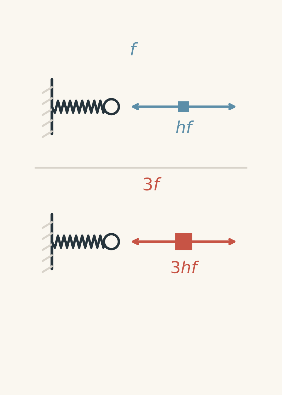
What happens when frequency increases?
Look at
\[ \Delta E=hf. \]
Planck’s constant \(h\) does not change. Therefore, if frequency doubles, the size of the quantum doubles.
A \(2f\) oscillator must gain or lose energy in steps of \(2hf\). It cannot absorb \(0.4hf\), or \(1.7hf\), because neither would leave it at an allowed energy.
This gives high-frequency radiation a built-in penalty. The higher the frequency, the larger the minimum energy packet involved.
03From Planck’s quanta to photons
There is an important historical detail that simplified HSC explanations can blur.
Planck introduced quantisation in 1900 to describe energy exchange by oscillators in matter. He did not initially claim that a travelling beam of light itself consisted of particles.
In 1905, Albert Einstein pushed the idea further by treating radiation itself as coming in discrete light quanta. In modern language, we call these quanta photons.
For HSC calculations, the practical rule is
\[ E=hf, \]
where \(E\) is the energy of one photon.
Because electromagnetic waves also satisfy
\[ c=f\lambda, \]
we can replace \(f\) with \(c/\lambda\):
\[ E=\frac{hc}{\lambda}, \]
where \(c=3.00\times10^8\ \text{m s}^{-1}\) is the speed of light in vacuum, and \(\lambda\) is wavelength in metres.
This immediately gives an important prediction:
- higher frequency \(\rightarrow\) greater photon energy,
- shorter wavelength \(\rightarrow\) greater photon energy.
Worked example: Find the energy of a blue-light photon
Blue light has a wavelength of \(450\ \text{nm}\). Calculate the energy of one photon.
Step 1
\[ 450\ \text{nm}=450\times10^{-9}\ \text{m} =4.50\times10^{-7}\ \text{m}. \]
Step 2
\[ E=\frac{hc}{\lambda}. \]
Step 3
\[ E= \frac{(6.63\times10^{-34})(3.00\times10^8)} {4.50\times10^{-7}} =4.42\times10^{-19}\ \text{J}. \]
Step 4
Each \(450\ \text{nm}\) photon carries approximately
\[ 4.42\times10^{-19}\ \text{J}. \]
That number looks tiny because a visible beam contains an enormous number of photons. Quantisation does not mean ordinary beams contain little total energy. It means the energy is exchanged in microscopic packets.
04Why quantisation fixes the ultraviolet catastrophe
Now return to the hot cavity.
In classical physics, energy could be distributed continuously among the electromagnetic modes. High-frequency modes were treated too generously, so the predicted spectrum kept rising towards shorter wavelengths.
Planck changed the rules.
For a low-frequency oscillator, \(hf\) is small. Relatively little energy is needed to move it from one allowed level to the next.
For a high-frequency oscillator, \(hf\) is large. At a fixed temperature, sufficiently large energy jumps become increasingly difficult to supply.
So high-frequency modes are strongly suppressed instead of receiving the large amount of energy predicted classically.
That produces a spectrum which rises, reaches a peak, and then falls at very high frequencies. The total emitted energy stays finite.
The important reasoning chain is:
\[ \text{higher }f \rightarrow \text{larger quantum }hf \rightarrow \text{harder to excite thermally} \rightarrow \text{less high-frequency radiation}. \]
Planck did not simply tweak the classical equation until the graph looked right. The successful model required a fundamentally different assumption about how energy could be exchanged.
05Quantised energy does not mean quantised frequency
A very tempting mistake is to hear “energy is quantised” and conclude that light is allowed to have only certain frequencies.
That is not what \(E=hf\) says.
Light can have many different frequencies. Once a particular frequency \(f\) is chosen, however, each photon at that frequency has the specific energy \(hf\).
There is another idea that can cause confusion here. A cavity can have particular allowed standing-wave frequencies because of its boundary conditions. That restriction comes from wave behaviour and the cavity’s geometry. It is different from Planck’s statement that energy exchange occurs in discrete amounts.
Keep the two ideas separate:
| Idea | What is restricted? | Why? |
|---|---|---|
| Cavity standing-wave modes | Possible frequencies in that cavity | Boundary conditions |
| Planck quantisation | Energy associated with a given oscillator frequency | Energy comes in steps of \(hf\) |
| Photon model | Energy of one photon at frequency \(f\) | \(E=hf\) |
06Photon energy and beam intensity are different ideas
Suppose you have a dim violet beam and a bright red beam.
Which has the more energetic individual photons?
The violet beam.
Which necessarily carries more total energy each second?
You cannot tell from the colour alone.
This distinction matters constantly in quantum physics. Frequency sets the energy of each photon:
\[ E_{\text{photon}}=hf. \]
The total energy of a simple monochromatic pulse also depends on how many photons it contains:
\[ E_{\text{total}}=NE_{\text{photon}}=Nhf, \]
where \(N\) is the number of photons.
Similarly, if a monochromatic source emits photons at a rate \(\dot N\), its power is
\[ P=\dot N hf. \]
So a brighter beam at the same frequency generally means more photons arriving per second, not more energy in each individual photon.
This is one of the most useful distinctions to carry into the photoelectric effect.
Worked example: How many photons are in a laser pulse?
A \(650\ \text{nm}\) laser produces \(2.00\ \text{mW}\) of power for \(3.00\ \text{ms}\). Estimate the number of photons emitted during the pulse.
Step 1
Convert the wavelength:
\[ 650\ \text{nm}=6.50\times10^{-7}\ \text{m}. \]
Then
\[ E_{\text{photon}} = \frac{hc}{\lambda} = \frac{(6.63\times10^{-34})(3.00\times10^8)} {6.50\times10^{-7}} = 3.06\times10^{-19}\ \text{J}. \]
Step 2
Power is energy transferred per unit time:
\[ P=\frac{E_{\text{pulse}}}{t}. \]
Therefore,
\[ E_{\text{pulse}}=Pt. \]
Using \(2.00\ \text{mW}=2.00\times10^{-3}\ \text{W}\) and \(3.00\ \text{ms}=3.00\times10^{-3}\ \text{s}\),
\[ E_{\text{pulse}} = (2.00\times10^{-3})(3.00\times10^{-3}) = 6.00\times10^{-6}\ \text{J}. \]
Step 3
\[ N = \frac{E_{\text{pulse}}}{E_{\text{photon}}} = \frac{6.00\times10^{-6}} {3.06\times10^{-19}} = 1.96\times10^{13}. \]
Step 4
The pulse contains about
\[ 1.96\times10^{13} \]
photons.
Each photon carries an extremely small amount of energy, but there are nearly twenty trillion of them in this short pulse. That is why macroscopic light can appear smoothly variable even though its microscopic energy exchanges are quantised.
07What actually changed in the model of light?
Planck’s work did not prove that the classical wave model was useless.
Light still diffracts. It still interferes. Maxwell’s electromagnetic wave theory still describes a huge range of observations extremely well.
What changed was the assumption that energy must always be exchanged continuously.
The classical picture says, roughly, “an oscillator can give radiation any amount of energy you like.”
Planck’s model says, “for an oscillator of frequency \(f\), allowed energy changes come in units related to \(hf\).”
Einstein’s photon model then makes the stronger statement that individual radiation quanta carry energy \(hf\).
So quantum theory did not simply replace “light is a wave” with “light is a particle”. The more accurate lesson is that classical waves alone are incomplete. Some interactions require a quantised description of energy.
08Questions and solutions
Question 1
A photon has a frequency of \(5.00\times10^{14}\ \text{Hz}\).
Calculate its energy.
Solution 1
The photon energy is \(3.32\times10^{-19}\ \text{J}\).
For a photon,
\[ E=hf. \]
Substituting,
\[ E = (6.63\times10^{-34})(5.00\times10^{14}) = 3.315\times10^{-19}\ \text{J}. \]
To three significant figures,
\[ E=3.32\times10^{-19}\ \text{J}. \]
The governing idea is that the frequency already tells us the energy of each individual photon. There is no need to use \(c=f\lambda\) unless a wavelength is required.
A common mistake is to think that \(5.00\times10^{14}\ \text{Hz}\) tells us how many photons arrive each second. It does not. Frequency describes the electromagnetic oscillation; photon arrival rate is a separate quantity.
Question 2
Two monochromatic light sources each have a power of \(1.00\ \text{mW}\).
Source A emits at \(400\ \text{nm}\), while source B emits at \(800\ \text{nm}\).
Calculate the photon emission rate of each source, and determine which source emits more photons each second.
Solution 2
The \(800\ \text{nm}\) source emits twice as many photons per second: approximately \(4.02\times10^{15}\ \text{s}^{-1}\), compared with \(2.01\times10^{15}\ \text{s}^{-1}\) for the \(400\ \text{nm}\) source.
First calculate the energy of a \(400\ \text{nm}\) photon:
\[ E_{400} = \frac{hc}{\lambda} = \frac{(6.63\times10^{-34})(3.00\times10^8)} {400\times10^{-9}} = 4.97\times10^{-19}\ \text{J}. \]
For \(800\ \text{nm}\),
\[ E_{800} = \frac{(6.63\times10^{-34})(3.00\times10^8)} {800\times10^{-9}} = 2.49\times10^{-19}\ \text{J}. \]
Power is energy transferred per second, so
\[ P=\dot N E_{\text{photon}}, \]
giving
\[ \dot N=\frac{P}{E_{\text{photon}}}. \]
For source A,
\[ \dot N_A = \frac{1.00\times10^{-3}} {4.97\times10^{-19}} = 2.01\times10^{15}\ \text{s}^{-1}. \]
For source B,
\[ \dot N_B = \frac{1.00\times10^{-3}} {2.49\times10^{-19}} = 4.02\times10^{15}\ \text{s}^{-1}. \]
Both sources transfer the same total energy each second because their powers are equal. The difference is how that energy is divided into quanta.
The tempting prediction is that the shorter-wavelength source must emit “more light” because its photons are more energetic. The missing constraint is equal power. If each \(400\ \text{nm}\) photon carries twice as much energy, only half as many photons are required each second.
Question 3
A pulse contains exactly \(3.00\times10^{12}\) photons. Every photon has a wavelength of either \(400\ \text{nm}\) or \(800\ \text{nm}\).
The pulse carries a total energy of \(9.95\times10^{-7}\ \text{J}\).
Determine the number of photons of each wavelength.
Solution 3
The pulse contains approximately \(1.00\times10^{12}\) photons at \(400\ \text{nm}\) and \(2.00\times10^{12}\) photons at \(800\ \text{nm}\).
From the previous relationships,
\[ E_{400}=4.97\times10^{-19}\ \text{J} \]
and
\[ E_{800}=2.49\times10^{-19}\ \text{J}. \]
Let \(x\) be the number of \(400\ \text{nm}\) photons and \(y\) the number of \(800\ \text{nm}\) photons.
The total photon count gives
\[ x+y=3.00\times10^{12}. \]
The total energy gives
\[ (4.97\times10^{-19})x + (2.49\times10^{-19})y = 9.95\times10^{-7}. \]
Using
\[ y=3.00\times10^{12}-x, \]
we obtain
\[ (4.97\times10^{-19})x + (2.49\times10^{-19})(3.00\times10^{12}-x) = 9.95\times10^{-7}. \]
Solving gives, to the precision of the supplied data,
\[ x\approx1.00\times10^{12}, \]
so
\[ y\approx2.00\times10^{12}. \]
A tempting shortcut is to divide the total energy by \(3.00\times10^{12}\) and treat that average as the energy of every photon. That would give an energy corresponding to a wavelength between \(400\) and \(800\ \text{nm}\).
But the question says every photon belongs to one of two discrete groups. An average energy describes the collection; it does not create a third type of photon.
Question 4
Consider two ideal Planck oscillators that can exchange energy only with each other.
Oscillator A has frequency \(f=4.00\times10^{14}\ \text{Hz}\), so its allowed energies are
\[ E_A=m hf, \]
where \(m\) is a non-negative integer.
Oscillator B has frequency
\[ \frac{3}{2}f, \]
so its allowed energies are
\[ E_B=n\,h\left(\frac{3}{2}f\right), \]
where \(n\) is a non-negative integer.
Initially, A has energy \(6hf\), and B has zero energy.
Assuming exact energy conservation and no other energy reservoir:
- What is the smallest non-zero amount of energy that can be transferred from A to B?
- What possible final energies can B have?
Solution 4
The smallest non-zero transfer is \(3hf=7.96\times10^{-19}\ \text{J}\), and B can finish with \(0\), \(3hf\), or \(6hf\).
A can lose energy only in integer multiples of \(hf\):
\[ \Delta E_A=m'hf, \]
where \(m'\) is a positive integer.
B can gain energy only in integer multiples of
\[ \frac{3}{2}hf. \]
For an allowed transfer, the amount lost by A must exactly equal the amount gained by B:
\[ m'hf = n'\left(\frac{3}{2}hf\right). \]
Cancel \(hf\):
\[ m'=\frac{3}{2}n'. \]
The smallest positive integers satisfying this equation are
\[ m'=3,\qquad n'=2. \]
Therefore,
\[ \Delta E_{\min}=3hf. \]
Numerically,
\[ \Delta E_{\min} = 3(6.63\times10^{-34})(4.00\times10^{14}) = 7.96\times10^{-19}\ \text{J}. \]
A begins with \(6hf\), so it can make either one transfer of \(3hf\) or a total transfer of \(6hf\) while remaining at an allowed level.
Therefore B’s possible final energies are
\[ 0,\qquad3hf,\qquad6hf. \]
The tempting answer is that B should be able to gain one of its own quanta, \(1.5hf\). B certainly has a level at that energy. But A has no way to lose exactly \(1.5hf\).
Energy conservation alone is not enough. The transfer must satisfy the quantisation rules of both systems simultaneously.
Question 5
A lossless black box receives \(4.00\times10^{15}\) photons per second, all with wavelength \(600\ \text{nm}\).
The output contains only \(600\ \text{nm}\) photons and \(300\ \text{nm}\) photons. The total output photon rate is \(3.00\times10^{15}\ \text{s}^{-1}\), and no other energy enters or leaves the box.
- Determine the output rate of \(300\ \text{nm}\) photons and \(600\ \text{nm}\) photons.
- What fraction of the incoming photons must participate in the energy conversion?
- A student divides the total output power by the total output photon rate and obtains an average photon energy corresponding to \(450\ \text{nm}\). They conclude that the output is effectively \(450\ \text{nm}\) light. Explain the error.
- The output then strikes an ideal detector that responds only when an individual photon has energy at least \(5.00\times10^{-19}\ \text{J}\). Assuming every qualifying photon is detected, calculate the detector’s count rate.
Solution 5
The output must contain \(1.00\times10^{15}\) photons per second at \(300\ \text{nm}\) and \(2.00\times10^{15}\) photons per second at \(600\ \text{nm}\). Half of the incoming photons participate in the conversion, the \(450\ \text{nm}\) conclusion is false, and the detector records \(1.00\times10^{15}\) counts per second.
Start with the energy of one \(600\ \text{nm}\) photon. Call it \(E\):
\[ E=\frac{hc}{600\times10^{-9}}. \]
A \(300\ \text{nm}\) photon has half the wavelength, so it has twice the energy:
\[ E_{300}=2E. \]
Let \(x\) be the number of \(300\ \text{nm}\) photons emitted per second and \(y\) the number of \(600\ \text{nm}\) photons emitted per second.
The measured output photon rate gives
\[ x+y=3.00\times10^{15}. \]
The input energy transferred each second is
\[ (4.00\times10^{15})E. \]
Because the box is lossless, output power must equal input power:
\[ 2Ex+Ey=(4.00\times10^{15})E. \]
Cancel \(E\):
\[ 2x+y=4.00\times10^{15}. \]
Subtracting
\[ x+y=3.00\times10^{15} \]
gives
\[ x=1.00\times10^{15}\ \text{s}^{-1}. \]
Therefore,
\[ y=2.00\times10^{15}\ \text{s}^{-1}. \]
Each \(300\ \text{nm}\) photon contains the energy of two \(600\ \text{nm}\) photons. With no external energy source, the required energy bookkeeping is therefore two incoming \(600\ \text{nm}\) photons for each \(300\ \text{nm}\) photon produced.
Producing
\[ 1.00\times10^{15} \]
high-energy photons each second therefore involves
\[ 2.00\times10^{15} \]
incoming photons each second.
The fraction participating is
\[ \frac{2.00\times10^{15}} {4.00\times10^{15}} =0.500, \]
or \(50.0\%\).
Now consider the student’s average-energy argument.
The average output energy per photon really is
\[ \frac{\text{total output energy per second}} {\text{total photons per second}} = \frac{4E}{3}. \]
Since \(E\) corresponds to \(600\ \text{nm}\), an energy of \(4E/3\) would correspond to
\[ \lambda = 600\ \text{nm}\times\frac{3}{4} = 450\ \text{nm}. \]
But that is only an average across the whole population. The actual output contains two groups: \(600\ \text{nm}\) photons and \(300\ \text{nm}\) photons. There need not be a single \(450\ \text{nm}\) photon present.
This becomes crucial for the detector.
For \(600\ \text{nm}\),
\[ E_{600} = \frac{(6.63\times10^{-34})(3.00\times10^8)} {600\times10^{-9}} = 3.32\times10^{-19}\ \text{J}. \]
This is below the detector threshold.
For \(300\ \text{nm}\),
\[ E_{300} = 6.63\times10^{-19}\ \text{J}, \]
which is above the threshold.
Therefore only the \(300\ \text{nm}\) photons produce counts:
\[ \text{count rate} = 1.00\times10^{15}\ \text{s}^{-1}. \]
This is the key trap. The average photon energy,
\[ \frac{4E}{3}\approx4.42\times10^{-19}\ \text{J}, \]
is below the detector threshold. If you replaced the real mixture with fictional \(450\ \text{nm}\) photons, you would predict no detections at all.
That prediction would be completely wrong.
Whenever an interaction depends on the energy of an individual quantum, an average over many photons can hide exactly the information that matters.
09What Planck’s idea lets you understand next
Once energy comes in quanta, several results that look strange classically become much easier to predict.
The photoelectric effect depends on photon energy \(hf\), not simply the total brightness of the beam. Atomic emission spectra make sense because atoms change between discrete energy levels. High-frequency radiation behaves differently from low-frequency radiation because its individual quanta carry more energy.
For thermal radiation, Planck’s model also explains why a spectrum has a finite peak rather than climbing forever. The next useful question is where that peak occurs. Wien’s displacement law connects that peak wavelength directly to temperature.
The decision rule to carry forward is simple: whenever a problem involves absorption, emission, or a threshold interaction, separate two questions. How much energy does each quantum carry? And how many quanta are involved? Classical physics tends to blend those into one continuous energy flow. Planck’s insight was that, microscopically, that distinction can change the prediction completely.