
How Particle Accelerators Test Relativity: HSC Physics
Learn why particles near the speed of light can gain substantial energy without much extra speed, and how their laboratory lifetimes test time dilation. Includes two worked examples and five questions with solutions, progressing from HSC applications to demanding conceptual challenges.
An electron is already travelling at \(0.99c\), where \(c\) is the speed of light in a vacuum. Predict what happens when an accelerator doubles its kinetic energy. Does its speed increase by a factor of \(\sqrt{2}\), as it would for a golf ball?
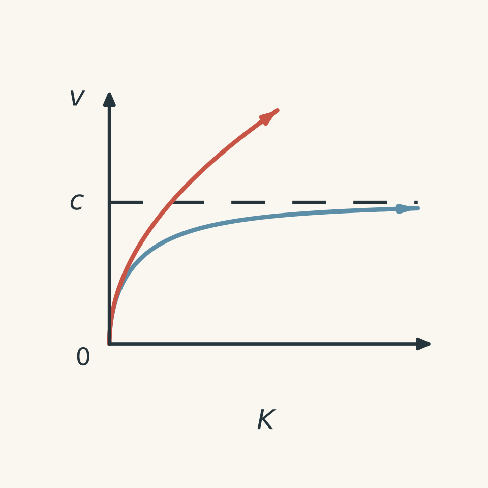
No. Its speed rises to about \(0.997c\), not \(1.40c\). The extra energy is real; the familiar relationship between energy and speed is what fails. Particle accelerators let us investigate that failure using measurements of energy, speed, and, for unstable particles, lifetime.
01Why extra energy barely changes the speed
An accelerating electric field transfers energy to a charged particle by doing work on it. Magnetic fields have a different job: they can steer the particle without increasing its speed. Keeping a beam going around a ring and increasing its energy are separate tasks. CERN
For a slowly moving golf ball, the kinetic energy is approximately \(K=\tfrac12m_0v^2\), where \(K\) is kinetic energy, \(m_0\) is rest mass, and \(v\) is speed. Doubling \(K\) therefore multiplies \(v\) by \(\sqrt{2}\).
That relationship is a low-speed approximation. Near the speed of light, a particle can gain a large amount of kinetic energy while gaining very little speed. We need a relationship that describes both regimes. Feynman Lectures
The energy scale that matters
A particle’s rest energy is \(E_0=m_0c^2\): the energy associated with its rest mass. Here, \(m_0\) is measured in kilograms, and we will use \(c=3.00\times10^8\ \mathrm{m\,s^{-1}}\).
Relativistic effects become important when the kinetic energy is no longer small compared with this rest energy.
The quantity connecting speed and energy is the Lorentz factor:
\[ \gamma=\frac{1}{\sqrt{1-v^2/c^2}}. \]
The symbol \(\gamma\), pronounced “gamma”, has no units. It equals \(1\) at rest and increases as \(v\) approaches \(c\).
The particle’s total energy \(E\) includes both rest energy and kinetic energy:
\[ E=\gamma E_0, \qquad K=E-E_0=(\gamma-1)E_0. \]
These are not two competing energy formulas. The second simply subtracts the energy the particle already has at rest. Feynman Lectures
For calculations, this gives a useful sequence:
\[ \gamma=1+\frac{K}{E_0}, \qquad v=c\sqrt{1-\frac{1}{\gamma^2}}. \]
When the question gives kinetic energy, include the \(+1\). When it gives total energy, use \(\gamma=E/E_0\) instead.
As \(v\) approaches \(c\), the denominator in the Lorentz factor approaches zero. Consequently, \(\gamma\), and therefore the required kinetic energy, increases without limit. A particle with non-zero rest mass cannot be accelerated to \(c\) using finite energy. CERN Videos
Rest mass is not increasing
Some questions use the term relativistic mass, defined as \(m_{\mathrm{rel}}=\gamma m_0\). This expresses the increasing total energy as a mass-equivalent quantity.
The particle’s rest mass \(m_0\) does not increase just because it moves faster. Also, replacing \(m_0\) with \(m_{\mathrm{rel}}\) in \(\tfrac12m_0v^2\) does not repair the classical kinetic-energy formula. Use \(K=(\gamma-1)m_0c^2\). Of Particular Significance
Worked example: How fast is a 1.50 MeV electron?
An electron has kinetic energy \(1.50\ \mathrm{MeV}\). Calculate its speed, and show why the classical kinetic-energy formula is unsuitable. Use the electron rest energy \(E_0=0.511\ \mathrm{MeV}\). NIST
Energy can be expressed in joules, written \(\mathrm J\), or megaelectronvolts, written \(\mathrm{MeV}\). The conversion is approximately \(1\ \mathrm{MeV}=1.60\times10^{-13}\ \mathrm J\). Here, keeping both energies in MeV makes their ratio straightforward.
Step 1
\[ \gamma =1+\frac{K}{E_0} =1+\frac{1.50\ \mathrm{MeV}}{0.511\ \mathrm{MeV}} =3.935. \]
The energy units cancel, as they should: \(\gamma\) is a pure number.
Step 2
\[ \begin{aligned} v &=c\sqrt{1-\frac{1}{\gamma^2}}\\ &=(3.00\times10^8)\sqrt{1-\frac{1}{3.935^2}}\\ &=2.90\times10^8\ \mathrm{m\,s^{-1}} =0.967c. \end{aligned} \]
The electron has substantial kinetic energy, but its speed remains below \(c\).
Step 3
Using \(E_0=m_0c^2\), the classical formula would give:
\[ \frac{v_{\mathrm{classical}}}{c} =\sqrt{\frac{2K}{E_0}} =\sqrt{\frac{2(1.50)}{0.511}} =2.42. \]
It predicts \(v_{\mathrm{classical}}=2.42c\). This is not evidence that the electron exceeds the speed of light. It shows that the low-speed approximation has been used outside its valid range.
02How an experiment separates speed from energy
In 1964, William Bertozzi reported measurements using electron pulses with energies from \(0.5\) to \(15\ \mathrm{MeV}\). The pulses passed a start pick-up, travelled along an \(8.4\ \mathrm m\) evacuated accelerator section, and struck an aluminium disc that produced a stop signal. The signal separation gave their average flight speed. At high energies, increasing the accelerator setting barely changed the flight time. Muj Optol
A weakness remained: an accelerator setting was not an independent measurement of the energy delivered.
Bertozzi therefore also measured the disc’s heating and the collected charge. The heating measured deposited energy; the charge established how many electrons delivered it. This showed that energy per electron increased even when speed changed little. The result supported the relativistic relationship rather than the classical one. Muj Optol
That experimental separation is essential. Calculating speed from the relativistic energy formula, then using that calculated speed to “confirm” the formula, would be circular reasoning.
A stronger test measures distance and flight time independently of energy. It also checks timing delays, energy losses, and particle number. More heat alone could mean more particles, not more energy per particle.
03Fast particles last longer on the laboratory clock
Unstable particles provide another kind of measurement.
Imagine a box of tiny stopwatches whose alarms go off at random. One alarm tells you very little, but thousands reveal a reliable average waiting time. Particle decay provides a statistical clock in a similar way.
The analogy has a limit: a particle contains neither a stopwatch nor a scheduled alarm. Its decay is random. The predictable quantity is the distribution of decay times across many identical particles. Massachusetts Institute of Technology
Now make a second prediction: if a fast beam barely gains speed when its energy increases, must the particles’ average travel distance before decay also barely increase?
No. Their laboratory lifetimes can increase substantially, allowing much longer journeys without much greater speed.
Proper lifetime and laboratory lifetime
The mean proper lifetime, \(\tau_0\), is the average lifetime measured in the particle’s rest frame.
For identical particles travelling at one constant speed, the mean lifetime measured in the laboratory is:
\[ \tau_{\mathrm{lab}}=\gamma\tau_0. \]
Both lifetimes are measured in units of time. A microsecond, written \(\mu\mathrm s\), is \(10^{-6}\ \mathrm s\).
The particle’s rest-frame decay behaviour has not changed. The laboratory assigns a longer time interval to that behaviour because the particle is moving relative to it. This is time dilation, not merely a delay in light reaching an observer. Massachusetts Institute of Technology
For the frame-selection method behind this equation, see tutorgum’s guide to proper time and the Lorentz factor.
What storage-ring measurements found
Muons are unstable particles with a mean proper lifetime of approximately \(2.20\ \mu\mathrm s\).
A 1977 CERN experiment measured muons circulating in a storage ring with \(\gamma\approx29.33\). Their measured laboratory mean lifetimes were about \(64.4\ \mu\mathrm s\), consistent with the relativistic prediction using the measured lifetime at rest. Nature
The evidence is not simply that some muons survived for a surprisingly long time. Individual decay times vary. The evidence is that the measured distribution of laboratory decay times had the mean lifetime predicted by time dilation.
Worked example: How far does an energetic muon travel?
A narrow muon beam has kinetic energy \(K=4.00E_0\) per muon and mean proper lifetime \(\tau_0=2.20\ \mu\mathrm s\). Calculate the beam’s speed, its mean laboratory lifetime, and its mean distance travelled before decay.
Assume constant speed in an evacuated straight beamline, with no losses other than decay.
Step 1
\[ \begin{aligned} \gamma&=1+\frac{K}{E_0}=1+4.00=5.00,\\ v&=c\sqrt{1-\frac{1}{5.00^2}} =0.9798c =2.939\times10^8\ \mathrm{m\,s^{-1}}. \end{aligned} \]
Step 2
\[ \tau_{\mathrm{lab}} =\gamma\tau_0 =5.00(2.20\ \mu\mathrm s) =11.0\ \mu\mathrm s. \]
Step 3
Let \(D\) be the mean distance travelled before decay.
\[ \begin{aligned} D&=v\tau_{\mathrm{lab}}\\ &=(2.939\times10^8)(11.0\times10^{-6})\\ &=3.23\times10^3\ \mathrm m =3.23\ \mathrm{km}. \end{aligned} \]
Without time dilation, using the same measured speed would predict only
\[ v\tau_0 =(2.939\times10^8)(2.20\times10^{-6}) =647\ \mathrm m. \]
Time dilation increases the mean travel distance by a factor of five. This is not a maximum range: some muons decay earlier, and others travel farther.
04One factor must explain all three measurements
For a beam of identical particles at one speed, relativity connects the measurements through:
\[ \gamma =\frac{1}{\sqrt{1-v^2/c^2}} =1+\frac{K}{E_0} =\frac{\tau_{\mathrm{lab}}}{\tau_0}. \]
This combines the energy and time-dilation relationships. Measure one quantity, use it to predict another, and compare that prediction with an independent measurement.
Near \(c\), speed changes become small even while energy and laboratory lifetime continue increasing strongly. A speed reported as “approximately \(c\)” therefore does not establish either the particle’s exact speed or its energy.
The qualification “at one speed” matters. A beam containing a mixture of energies must be treated as a mixture, rather than automatically assigning one Lorentz factor to every particle.
Counting survivors, rather than treating lifetime as a deadline
For the questions below, use the usual exponential decay model:
\[ S(t)=\frac{N(t)}{N_0} =\exp\left(-\frac{t}{\gamma\tau_0}\right). \]
Here, \(N_0\) is the initial particle count, \(N(t)\) is the expected count remaining after laboratory time \(t\), and \(S(t)\) is the surviving fraction. The function \(\exp(x)\) means \(e^x\), where \(e\approx2.718\). Massachusetts Institute of Technology
After one mean laboratory lifetime, the surviving fraction is \(\exp(-1)\approx0.368\). About \(37\%\) remain-not zero, and not half.
When speed changes, calculate the proper time accumulated during each stage. Write the total as \(u\):
\[ u=\frac{\Delta t_1}{\gamma_1} +\frac{\Delta t_2}{\gamma_2} +\cdots, \qquad S=\exp\left(-\frac{u}{\tau_0}\right). \]
Each \(\Delta t\) is a laboratory time interval, and its subscript identifies the stage. The corresponding \(\gamma\) belongs to that stage. This follows by applying time dilation separately to each interval.
At rest, \(\gamma=1\), so waiting for one laboratory microsecond adds one microsecond of proper time.
05Questions and solutions
The experiments below are idealised. Ignore collisions, radiation losses, and detector inefficiency unless stated otherwise. Use \(c=3.00\times10^8\ \mathrm{m\,s^{-1}}\).
Question 1
An electron travels at \(0.800c\). Its rest energy is \(0.511\ \mathrm{MeV}\).
Calculate its Lorentz factor and kinetic energy. State whether its rest mass has increased.
Solution 1
The Lorentz factor is \(1.67\), the kinetic energy is \(0.341\ \mathrm{MeV}\), and the rest mass is unchanged.
\[ \begin{aligned} \gamma &=\frac{1}{\sqrt{1-0.800^2}} =1.667,\\ K &=(\gamma-1)E_0\\ &=(1.667-1)(0.511\ \mathrm{MeV})\\ &=0.341\ \mathrm{MeV}. \end{aligned} \]
The total energy is larger than the rest energy, but the particle has not acquired a larger rest mass. Calling \(\gamma m_0\) its relativistic mass is a different naming convention, not a change in \(m_0\).
Question 2
Two electron pulses are completely stopped in a calorimeter. Assume all their kinetic energy becomes measured thermal energy.
| Measurement | Pulse A | Pulse B |
|---|---|---|
| Number of electrons | \(1.00\times10^8\) | \(2.00\times10^8\) |
| Deposited thermal energy | \(1.60\times10^{-4}\ \mathrm J\) | \(6.40\times10^{-4}\ \mathrm J\) |
Before reaching the calorimeter, each pulse crosses a \(9.00\ \mathrm m\) field-free timing section. Both flight times are reported as \(30\ \mathrm{ns}\), rounded to the nearest \(1\ \mathrm{ns}\). A nanosecond is \(10^{-9}\ \mathrm s\).
Determine the kinetic energy per electron in each pulse and the flight time predicted by relativity. Evaluate the claims that Pulse B’s electrons have four times the kinetic energy and that both beams have reached \(c\).
Use \(E_0=0.511\ \mathrm{MeV}\) and \(1\ \mathrm{MeV}=1.60\times10^{-13}\ \mathrm J\).
Solution 2
The kinetic energy per electron doubles, from \(10.0\) to \(20.0\ \mathrm{MeV}\). Both flight times can round to \(30\ \mathrm{ns}\) without either beam reaching \(c\).
Let \(H\) be deposited thermal energy and \(n\) the number of electrons. The kinetic energy per electron is \(K=H/n\):
\[ \begin{aligned} K_A &=\frac{1.60\times10^{-4}}{1.00\times10^8} =1.60\times10^{-12}\ \mathrm J =10.0\ \mathrm{MeV},\\ K_B &=\frac{6.40\times10^{-4}}{2.00\times10^8} =3.20\times10^{-12}\ \mathrm J =20.0\ \mathrm{MeV}. \end{aligned} \]
The calorimeter received four times as much energy, but twice as many electrons delivered it. Ignoring particle number would give the wrong energy per electron.
The Lorentz factors are:
\[ \gamma_A=1+\frac{10.0}{0.511}=20.57, \qquad \gamma_B=1+\frac{20.0}{0.511}=40.14. \]
For timing-section length \(L\), the flight time is
\[ \Delta t=\frac{L}{v} =\frac{L}{c\sqrt{1-1/\gamma^2}}. \]
Therefore,
\[ \begin{aligned} \Delta t_A &=\frac{9.00}{(3.00\times10^8)\sqrt{1-1/20.57^2}} \approx30.04\ \mathrm{ns},\\ \Delta t_B &=\frac{9.00}{(3.00\times10^8)\sqrt{1-1/40.14^2}} \approx30.01\ \mathrm{ns}. \end{aligned} \]
Both round to \(30\ \mathrm{ns}\) at the stated resolution. The instrument cannot distinguish these small differences; it has not established exact equality with \(c\).
The combination of greater energy per electron and nearly unchanged flight time is the relevant observation.
Question 3
A bunch initially contains \(N_0\) identical unstable particles. Each has rest energy \(E_0\), mean proper lifetime \(2.00\ \mu\mathrm s\), and kinetic energy \(4E_0\).
After \(10.0\ \mu\mathrm s\) of laboratory time, every surviving particle is rapidly slowed to kinetic energy \(E_0\). The slowing takes negligible time and does not change the particles’ intrinsic decay behaviour.
Find the fraction of the original bunch remaining at laboratory time \(14.0\ \mu\mathrm s\).
Also determine the mean remaining laboratory lifetime immediately after slowing. Explain why it is not zero, even though the bunch has already travelled for one initial mean laboratory lifetime.
Solution 3
At \(14.0\ \mu\mathrm s\), \(13.5\%\) of the original bunch remains. Immediately after slowing, the surviving particles have a mean remaining laboratory lifetime of \(4.00\ \mu\mathrm s\).
The two kinetic energies give different Lorentz factors:
\[ \gamma_1=1+\frac{4E_0}{E_0}=5, \qquad \gamma_2=1+\frac{E_0}{E_0}=2. \]
The total proper time accumulated by \(14.0\ \mu\mathrm s\) is:
\[ \begin{aligned} u &=\frac{10.0\ \mu\mathrm s}{5} +\frac{4.00\ \mu\mathrm s}{2}\\ &=4.00\ \mu\mathrm s,\\ \frac{N}{N_0} &=\exp\left(-\frac{4.00}{2.00}\right) =\exp(-2) =0.135. \end{aligned} \]
Slowing the particles makes them accumulate proper time faster per laboratory microsecond. It therefore increases their laboratory decay rate.
However, a mean lifetime is not a time allowance that gets used up. In the exponential model, surviving an earlier interval does not shorten the expected remaining proper lifetime.
To see this, let \(w\) be an additional proper-time interval. For particles that have already survived proper time \(u\), the fraction surviving a further \(w\) is:
\[ \frac{\exp[-(u+w)/\tau_0]}{\exp(-u/\tau_0)} =\exp(-w/\tau_0). \]
The previous age cancels. Their mean remaining proper lifetime is still \(\tau_0\), so after slowing:
\[ \tau_{\mathrm{remaining,lab}} =\gamma_2\tau_0 =2(2.00\ \mu\mathrm s) =4.00\ \mu\mathrm s. \]
This does not bring back particles that already decayed. It describes the future behaviour of those still present.
Question 4
Identical charged, unstable particles start at rest at a source. Their mean proper lifetime is \(2.00\ \mu\mathrm s\), and their rest energy is \(E_0\).
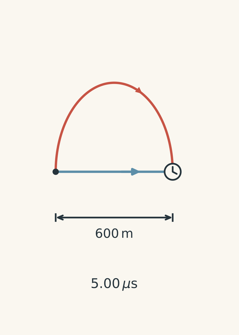
They must be at rest at a detector \(600\ \mathrm m\) from the source at laboratory time \(5.00\ \mu\mathrm s\). At no point may their kinetic energy exceed \(\tfrac23E_0\).
A proposed route accelerates them to the permitted maximum speed, sends them straight to the detector, stops them on arrival, and waits until the deadline.
Calculate the surviving fraction for this proposal. Then find the greatest possible surviving fraction under the same energy cap and deadline. Describe a route that achieves it, and justify why no allowed schedule can do better.
Assume evacuated routes of any required length are available. Stationary magnetic fields can steer the particles without changing their kinetic energy, and acceleration and stopping take negligible time.
Solution 4
The straight-route-and-wait proposal preserves \(13.5\%\) of the particles. The maximum is \(22.3\%\), achieved by travelling at \(0.800c\) throughout the \(5.00\ \mu\mathrm s\) interval along a \(1.20\ \mathrm{km}\) route, then stopping at the detector.
First, translate the energy cap into a speed cap:
\[ \begin{aligned} \gamma_{\max} &=1+\frac{(2/3)E_0}{E_0} =\frac53,\\ v_{\max} &=c\sqrt{1-\frac{1}{(5/3)^2}} =0.800c. \end{aligned} \]
For the straight route, the flight takes:
\[ t_{\mathrm{flight}} =\frac{600}{0.800(3.00\times10^8)} =2.50\ \mu\mathrm s. \]
That leaves \(2.50\ \mu\mathrm s\) waiting at rest. The accumulated proper time and surviving fraction are:
\[ \begin{aligned} u_{\mathrm{direct}} &=\frac{2.50}{5/3}+2.50 =4.00\ \mu\mathrm s,\\ S_{\mathrm{direct}} &=\exp\left(-\frac{4.00}{2.00}\right) =0.135. \end{aligned} \]
The tempting strategy is to minimise flight time. But the detector counts survivors at a fixed deadline, not immediately on arrival. Arriving early creates a waiting period during which the particle clocks accumulate proper time at the full laboratory rate.
Moving that waiting period to the source would not help. Waiting at rest adds the same proper time at either location.
Now consider the best possible schedule. Since \(\gamma\) can never exceed \(5/3\), every laboratory interval contributes at least \(3/5\) as much proper time. Over the whole journey:
\[ u\geq\frac{5.00\ \mu\mathrm s}{5/3} =3.00\ \mu\mathrm s. \]
Smaller accumulated proper time means greater survival. Hence:
\[ S\leq\exp\left(-\frac{3.00}{2.00}\right) =0.223. \]
This bound can be reached by remaining at the maximum speed for the entire interval. The required path length is:
\[ \begin{aligned} L &=v_{\max}t\\ &=0.800(3.00\times10^8)(5.00\times10^{-6})\\ &=1.20\times10^3\ \mathrm m. \end{aligned} \]
A curved route can have this length while connecting endpoints only \(600\ \mathrm m\) apart. Magnetic steering changes direction without requiring greater kinetic energy.
The longer route wins because it replaces waiting at rest with time spent moving. Both strategies finish at the same place, time, and energy, but the particles accumulate different proper times along the way.
Question 5
An accelerator produces large, identically prepared bunches of one unstable particle species. Each particle has rest energy \(E_0\) and mean proper lifetime \(\tau_0\).
After leaving the accelerator, every particle maintains its speed and is followed until decay. Measurements on separate, identically prepared bunches establish:
- The initial mean kinetic energy is \(4E_0\).
- The mean laboratory time from release to decay is \(5\tau_0\).
A report concludes that every particle has \(\gamma=5\) and therefore travels at one common speed.
A rival explanation is that half the particles have \(\gamma=2\), while half have \(\gamma=8\).
Determine whether the rival explanation fits both measurements. For that mixture, calculate the mean kinetic energy of the surviving particles at laboratory time \(4\tau_0\), and explain whether its change requires energy transfer to the survivors.
Finally, let \(S(t)\) be the fraction of the original bunch surviving to laboratory time \(t\). Develop a test using \(S(T)\) and \(S(2T)\), for any positive interval \(T\), that distinguishes a single-speed beam from the proposed mixture. Treat statistical fluctuations as negligible.
Solution 5
The rival mixture fits both measurements, so the report has not established a common speed. At \(4\tau_0\), the survivors’ mean kinetic energy is approximately \(5.91E_0\), even though no surviving particle has gained energy.
A single-speed beam satisfies \(S(2T)=[S(T)]^2\). The proposed mixture instead satisfies \(S(2T)>[S(T)]^2\).
First, examine the two initial averages.
Particles with \(\gamma=2\) have kinetic energy \(E_0\) and mean laboratory lifetime \(2\tau_0\). Those with \(\gamma=8\) have kinetic energy \(7E_0\) and mean laboratory lifetime \(8\tau_0\). Thus:
\[ \begin{aligned} \text{Mean kinetic energy} &=\frac{E_0+7E_0}{2} =4E_0,\\ \text{Mean laboratory lifetime} &=\frac{2\tau_0+8\tau_0}{2} =5\tau_0. \end{aligned} \]
Both reported averages are reproduced exactly.
Yet the two speeds are \(0.866c\) and \(0.992c\), obtained from \(v=c\sqrt{1-1/\gamma^2}\). Neither equals the single speed \(0.980c\) inferred from \(\gamma=5\).
The error is treating an average over different particles as a property possessed by every particle.
Next, follow the mixture through decay. At laboratory time \(4\tau_0\), let \(s_2\) and \(s_8\) be the surviving fractions within the two original groups:
\[ \begin{aligned} s_2 &=\exp\left(-\frac{4\tau_0}{2\tau_0}\right) =\exp(-2) =0.1353,\\ s_8 &=\exp\left(-\frac{4\tau_0}{8\tau_0}\right) =\exp(-0.5) =0.6065. \end{aligned} \]
The groups started with equal numbers, but they no longer contain equal numbers. The surviving high-energy group is much larger.
The mean kinetic energy among survivors must therefore be weighted by the surviving counts:
\[ \begin{aligned} \overline K_{\mathrm{surv}} &=\frac{s_2E_0+s_8(7E_0)}{s_2+s_8}\\ &=\frac{0.1353+7(0.6065)}{0.1353+0.6065}E_0\\ &=5.91E_0. \end{aligned} \]
Here, \(\overline K_{\mathrm{surv}}\) means the average kinetic energy of particles still undecayed.
No surviving particle has gained energy. Instead, lower-energy particles have been removed from the sample more rapidly by decay. The average describes a changing selection of particles; it is not the total energy of a closed system. Energy conservation applies when the decay products are included too.
Finally, construct the two-interval test.
For a single-speed beam, surviving each interval \(T\) has the same fractional effect:
\[ S(T)=\exp\left(-\frac{T}{\gamma\tau_0}\right), \qquad S(2T)=[S(T)]^2. \]
For the mixture, define the subgroup survival fractions over one interval as
\[ a=\exp\left(-\frac{T}{2\tau_0}\right), \qquad b=\exp\left(-\frac{T}{8\tau_0}\right). \]
Then:
\[ \begin{aligned} S(T)&=\frac{a+b}{2},\\ S(2T)&=\frac{a^2+b^2}{2},\\ S(2T)-[S(T)]^2 &=\frac{a^2+b^2}{2} -\left(\frac{a+b}{2}\right)^2\\ &=\frac{(a-b)^2}{4}>0. \end{aligned} \]
The inequality is strict because \(a\neq b\) whenever \(T>0\).
Physically, the first interval preferentially removes lower-energy particles. The second interval therefore starts with a population richer in long-lived, high-energy particles, so it retains a larger fraction of its starting population.
Both initial averages can look perfectly consistent with one Lorentz factor while the full decay curve reveals that no single factor describes the whole beam.
06What this lets you understand next
For detector placement, the important quantity is not just how close the particles are to \(c\). It is how much proper time they accumulate before reaching the detector, and how that varies across the beam.
For a straight, constant-speed beam, the same journey can also be described from the particle’s rest frame. Its proper lifetime stays unchanged; the laboratory apparatus is moving and its length along the motion is contracted. That is the next connection developed in tutorgum’s guide to length contraction: a different frame must explain the same survival outcome.