
Incomplete Flux Linkage and Leakage Flux in Transformers
Learn why real transformers do not achieve perfect flux linkage, how leakage flux affects induced emf, and how transformer design can improve magnetic coupling.
A 10:1 transformer connected to 240 V suggests a neat prediction: 24 V on the secondary. But that prediction quietly assumes something important. It assumes the changing magnetic flux responsible for the primary emf also links the secondary winding.
Now suppose some of the magnetic field loops around the primary winding and closes without passing through the secondary. The turns ratio has not changed. Should the secondary still behave like the ideal transformer? No. The two coils are no longer sharing all of the same changing flux.
That missing shared flux is the idea behind leakage flux.
01The turns ratio depends on shared flux
Start with Faraday’s law. A changing magnetic flux through a coil induces an emf:
\[
\varepsilon=-N\frac{\Delta \Phi}{\Delta t}
\]
where:
- \(\varepsilon\) is the induced emf in volts (V),
- \(N\) is the number of turns,
- \(\Delta \Phi\) is the change in magnetic flux through each turn in webers (Wb), and
- \(\Delta t\) is the time interval in seconds (s).
The negative sign comes from Lenz’s law and tells us the direction of the induced emf. When we only need the magnitude, we can work with absolute values.
If magnetic flux itself is still a bit slippery, revise Magnetic Flux for HSC Physics: Using Φ = BA cos θ first.
For an ideal transformer, the same changing core flux \(\Phi_m\) links every turn of both windings. So
\[
|\varepsilon_p|=N_p\left|\frac{\Delta \Phi_m}{\Delta t}\right|
\]
and
\[
|\varepsilon_s|=N_s\left|\frac{\Delta \Phi_m}{\Delta t}\right|.
\]
Here, \(N_p\) and \(N_s\) are the numbers of primary and secondary turns.
The changing-flux term is identical in both equations, so it cancels:
\[
\frac{|\varepsilon_s|}{|\varepsilon_p|}
=
\frac{N_s}{N_p}.
\]
That is the familiar ideal transformer relationship explained in Ideal Transformer Voltage and Turns Ratio for HSC Physics.
But notice what made the cancellation possible: both windings had to link the same changing flux.
02What leakage flux actually is
Magnetic field lines form closed loops. A ferromagnetic transformer core gives them a much easier path than air does, so most of the flux follows the core.
Most is not the same as all.
Some magnetic flux can form a smaller loop near one winding instead of following the core far enough to link the other winding. This is leakage flux.
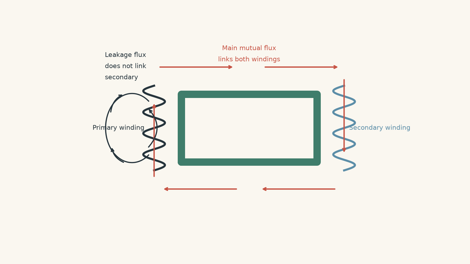
A useful mental picture is a train loop with two stations. The main, or mutual, flux follows the route past both the primary and secondary stations. Leakage flux takes a local siding near one station and rejoins without ever passing the other.
The picture helps with geometry, but don’t push it too far. Magnetic flux is not a stream of little objects travelling around the core.
Mutual flux and leakage flux
It helps to separate the field into two ideas.
Mutual flux links both windings. This is the flux that transfers electromagnetic effects from one winding to the other.
Leakage flux links one winding without fully linking the other.
When the secondary is supplying a load, current also flows through the secondary winding. That current produces its own magnetic field, so secondary leakage flux can exist as well.
A transformer therefore does not literally have one perfectly confined magnetic field. The useful ideal model treats it that way because, in a well-designed transformer, the mutual flux dominates.
03Flux linkage is the quantity Faraday’s law really cares about
There is a slightly more precise way to describe the problem.
For a coil, flux linkage is written as \(\lambda\). If all \(N\) turns link the same magnetic flux \(\Phi\),
\[
\lambda=N\Phi.
\]
Faraday’s law can then be written as
\[
\varepsilon=-\frac{\Delta \lambda}{\Delta t}.
\]
This matters because a winding with poor coupling may not have every turn linking exactly the same flux.
In the most general case,
\[
\lambda=\Phi_1+\Phi_2+\Phi_3+\cdots+\Phi_N,
\]
where \(\Phi_1,\Phi_2,\ldots\) are the fluxes linking the individual turns.
For a normal HSC calculation, you will usually be given a simpler situation where every secondary turn links some stated fraction of the relevant flux. Suppose that fraction is \(f\), where \(0\leq f\leq1\). Then
\[
\Phi_{\text{linked}}=f\Phi
\]
and
\[
|\varepsilon_s|
=
N_s f\left|\frac{\Delta\Phi}{\Delta t}\right|.
\]
If \(f=1\), all of that flux links the secondary. If \(f=0.94\), 94% links it and 6% follows leakage paths.
This \(f\) is a useful calculation model when a question explicitly gives a percentage of flux linkage. Do not automatically multiply every real transformer voltage ratio by a guessed leakage percentage. In an actual transformer, winding resistance, core behaviour, leakage inductance, load current, and the applied primary voltage all interact.
Worked example: Finding emf with incomplete flux linkage
A 250-turn secondary winding is exposed to a primary-produced magnetic flux that changes from \(0.80\text{ mWb}\) to \(0.20\text{ mWb}\) in \(4.0\text{ ms}\). Only 92% of this changing flux links each secondary turn. Find the magnitude of the average induced emf.
Step 1
\[
|\Delta\Phi|
=
|0.20-0.80|\text{ mWb}
=
0.60\text{ mWb}
=
6.0\times10^{-4}\text{ Wb}.
\]
Step 2
\[
|\Delta\Phi_{\text{linked}}|
=
0.92(6.0\times10^{-4})
=
5.52\times10^{-4}\text{ Wb}.
\]
Step 3
\[
|\varepsilon_s|
=
N_s\frac{|\Delta\Phi_{\text{linked}}|}{\Delta t}
=
250
\frac{5.52\times10^{-4}}{4.0\times10^{-3}}
=
34.5\text{ V}.
\]
The average induced emf is \(34.5\text{ V}\).
If all of the changing flux had linked the secondary, the result would have been
\[
250
\frac{6.0\times10^{-4}}{4.0\times10^{-3}}
=
37.5\text{ V}.
\]
The missing \(3.0\text{ V}\) in this simplified comparison comes from the incomplete flux linkage.
Worked example: Separating incomplete linkage from resistance
A loaded transformer has a 300-turn secondary. The changing mutual flux has an instantaneous rate of change of \(0.080\text{ Wb s}^{-1}\), and 97% of that flux links the secondary winding.
The secondary current is \(2.0\text{ A}\), and the secondary winding resistance is \(0.35\,\Omega\). For this calculation, neglect phase effects and other internal voltage drops.
Find the induced secondary emf and the approximate terminal voltage.
Step 1
\[
\left|\frac{d\Phi_{\text{linked}}}{dt}\right|
=
0.97(0.080)
=
0.0776\text{ Wb s}^{-1}.
\]
Step 2
\[
|\varepsilon_s|
=
N_s
\left|\frac{d\Phi_{\text{linked}}}{dt}\right|
=
300(0.0776)
=
23.28\text{ V}.
\]
So the winding has an induced emf of about \(23.3\text{ V}\).
Step 3
\[
V_R=IR=(2.0)(0.35)=0.70\text{ V}.
\]
Step 4
\[
V_{\text{terminal}}
\approx
23.28-0.70
=
22.58\text{ V}.
\]
So the terminal voltage is approximately \(22.6\text{ V}\) under the stated assumptions.
There are two different non-ideal effects here. Incomplete linkage affected the induced emf itself. The winding resistance then produced another voltage drop when current flowed.
Calling both of them “flux leakage” would hide the physics.
04Why transformer design changes the coupling
Coupling describes how effectively the changing magnetic field produced by one winding links the other winding.
Strong coupling means most of the relevant changing flux is shared. Weak coupling means more of it forms local leakage paths.
You can now predict the basic design strategy. If leakage flux is field that escapes into paths that miss the other winding, a good transformer should make the shared path magnetically easy and keep the two windings close to that path.
| Design change | Effect on coupling | Why |
|---|---|---|
| Use a high-permeability ferromagnetic core | Usually improves it | The core provides a low-reluctance path that concentrates flux |
| Use a closed magnetic core | Improves it | Flux can complete its magnetic path mainly through the core instead of through air |
| Place primary and secondary windings close together | Improves it | Fewer local field paths can link one winding while missing the other |
| Put windings concentrically on the same core limb | Often improves it strongly | The two windings occupy nearly the same magnetic region |
| Interleave sections of the primary and secondary | Can further reduce leakage | The magnetic separation between corresponding winding sections is reduced |
| Minimise unnecessary air gaps | Usually improves it | Air has much greater magnetic reluctance than a ferromagnetic core |
| Laminate the core | Mainly reduces eddy-current losses | Lamination is primarily an efficiency strategy, not the main method for reducing leakage flux |
| Use thicker winding wire | Reduces copper resistance | It can reduce \(I^2R\) loss but does not directly guarantee better magnetic coupling |
The distinction in the final two rows is important.
A student might reason, “Laminated cores make transformers more efficient, so laminations must stop leakage flux.” It sounds plausible because both are examples of non-ideal transformer behaviour.
But laminations mainly attack a different problem. A changing magnetic flux can induce unwanted eddy currents inside the conducting core. Dividing the core into insulated laminations makes those current loops harder to form.
Leakage flux is mainly a magnetic geometry and coupling problem.
05Why putting the windings closer helps
Imagine the primary and secondary wound on opposite sides of a large core window. Most flux still follows the core, but there is plenty of space for local fields around each winding.
Now move the windings onto the same core limb and place one concentrically around the other.
Before reading on, predict what happens to the amount of flux that can link one winding without linking the other.
It decreases.
The two windings now occupy almost the same magnetic region. A field that threads one is much more likely to thread the other as well.
This does not mean engineers simply squash the windings together as tightly as possible. Real transformers need electrical insulation, cooling, mechanical strength, and safe separation between different voltages. Good design is a compromise, not a contest to make the smallest gap imaginable.
06Leakage flux is not energy being “used up”
Another tempting picture is that magnetic flux leaves the primary, some of it transfers energy to the secondary, and the rest is somehow wasted.
Flux is not fuel.
A secondary winding does not consume magnetic flux. What matters is whether the changing magnetic field links the winding strongly enough to induce the required emf.
The phrase “leakage flux” describes the path and linkage of the magnetic field, not a substance escaping from a container.
07Better coupling does not automatically mean a perfect transformer
Suppose two windings have almost perfect flux linkage. Is the transformer now ideal?
Not necessarily.
It may still have:
- copper resistance in its windings,
- eddy-current losses in its core,
- hysteresis losses,
- heating,
- core saturation under unsuitable operating conditions, or
- load-dependent voltage drops.
Better coupling removes one source of non-ideal behaviour. It does not remove all of them.
This becomes especially important under load. Leakage flux is associated with leakage inductance, which can contribute to a voltage drop as current changes. That is one reason a real transformer’s terminal voltage can fall when a load draws more current.
08Questions and solutions
Question 1
A secondary coil has 300 turns. The magnetic flux associated with the primary changes by \(0.40\text{ mWb}\) in \(4.0\text{ ms}\). Only 90% of the changing flux links each secondary turn.
Calculate the magnitude of the average induced emf in the secondary.
Solution 1
The average induced emf is \(27\text{ V}\).
Only 90% of the stated flux change links the secondary, so
\[
|\Delta\Phi_{\text{linked}}|
=
0.90(0.40\times10^{-3})
=
3.6\times10^{-4}\text{ Wb}.
\]
Faraday’s law gives
\[
|\varepsilon|
=
N\frac{|\Delta\Phi_{\text{linked}}|}{\Delta t}
=
300
\frac{3.6\times10^{-4}}{4.0\times10^{-3}}
=
27\text{ V}.
\]
The tempting mistake is to put the full \(0.40\text{ mWb}\) into Faraday’s law. That would assume complete flux linkage even though the question explicitly tells us that 10% of the changing flux does not link the secondary.
Question 2
A 500-turn secondary is placed on a transformer core. During a particular \(2.0\text{ ms}\) interval, the magnitude of the total relevant core-flux change is \(0.30\text{ mWb}\).
In the original arrangement, only \(0.22\text{ mWb}\) of this change links each secondary turn. After the windings are rearranged concentrically on the same core limb, \(0.29\text{ mWb}\) links each turn.
Calculate:
- the percentage of the changing flux that fails to link the secondary before and after the rearrangement,
- the average secondary emf in each arrangement, and
- the average emf that would occur with complete linkage.
Explain why simply laminating the original core would not necessarily produce the same improvement.
Solution 2
The leakage fraction falls from about \(26.7\%\) to \(3.3\%\), while the average induced emf rises from \(55.0\text{ V}\) to \(72.5\text{ V}\). Complete linkage would give \(75.0\text{ V}\).
Before the rearrangement, the fraction linked is
\[
\frac{0.22}{0.30}=0.733.
\]
So the fraction failing to link is
\[
1-0.733=0.267,
\]
or approximately \(26.7\%\).
After rearrangement,
\[
\frac{0.29}{0.30}=0.967,
\]
so the leakage fraction is
\[
1-0.967=0.033,
\]
or about \(3.3\%\).
For the original arrangement,
\[
|\varepsilon_{\text{before}}|
=
N\frac{|\Delta\Phi_{\text{linked}}|}{\Delta t}
=
500
\frac{0.22\times10^{-3}}{2.0\times10^{-3}}
=
55.0\text{ V}.
\]
After rearrangement,
\[
|\varepsilon_{\text{after}}|
=
500
\frac{0.29\times10^{-3}}{2.0\times10^{-3}}
=
72.5\text{ V}.
\]
With complete linkage,
\[
|\varepsilon_{\text{complete}}|
=
500
\frac{0.30\times10^{-3}}{2.0\times10^{-3}}
=
75.0\text{ V}.
\]
The important design change is the reduced magnetic separation between the windings. Concentric windings are more likely to link the same magnetic field.
The tempting route is to say that any change known to “improve transformers” must improve coupling. Lamination mainly suppresses eddy currents in the core. Unless it also changes the magnetic geometry or effective core properties in a relevant way, it does not directly solve the large leakage path caused by poorly positioned windings.
Question 3
An \(800:80\) transformer is connected to a \(240\text{ V}\) AC supply.
The ideal turns ratio suggests a secondary voltage of \(24.0\text{ V}\). The measured no-load secondary voltage is \(23.8\text{ V}\).
When a \(6.0\,\Omega\) resistive load is connected, the terminal voltage falls to \(22.2\text{ V}\), and the secondary current is \(3.70\text{ A}\). The secondary winding resistance is \(0.20\,\Omega\).
Assume, for this estimate, that the measured no-load voltage already contains the effects present before the load is attached, and treat the load-dependent voltage drops as scalar quantities.
Determine how much of the additional voltage decrease after connecting the load can be accounted for by secondary winding resistance. What voltage decrease remains for other load-dependent effects, including leakage-related effects and primary winding drops?
Explain why it would be incorrect to describe the entire difference between \(24.0\text{ V}\) and \(22.2\text{ V}\) as leakage flux.
Solution 3
Secondary copper resistance accounts for \(0.74\text{ V}\) of the \(1.60\text{ V}\) load-dependent decrease, leaving about \(0.86\text{ V}\) for the other effects included in the simplified model.
The no-load secondary voltage is \(23.8\text{ V}\). Once the load is connected, it becomes \(22.2\text{ V}\).
So the additional decrease associated with loading is
\[
\Delta V_{\text{load}}
=
23.8-22.2
=
1.6\text{ V}.
\]
The secondary winding’s resistive drop is
\[
V_R=IR=(3.70)(0.20)=0.74\text{ V}.
\]
The remainder is therefore
\[
1.60-0.74=0.86\text{ V}.
\]
Under the assumptions in the question, that \(0.86\text{ V}\) represents the other load-dependent effects that have not been separately specified. These can include effects associated with leakage inductance and voltage drops in the primary winding.
The tempting argument is
\[
24.0-22.2=1.8\text{ V},
\]
followed by the claim that the whole \(1.8\text{ V}\) is caused by leakage flux.
That cannot be justified.
First, the transformer was already at \(23.8\text{ V}\) before the load was connected. Second, once current flows, the known secondary resistance alone causes a \(0.74\text{ V}\) drop. Leakage is only one of several non-ideal effects.
If the windings were moved closer while their resistance stayed unchanged, the leakage-related part of the voltage drop should decrease. The copper drop would not automatically disappear. In a real circuit, the changed terminal voltage could also change the current, so a fully precise prediction would require recalculating the complete loaded circuit.
Question 4
A 200-turn secondary winding has been constructed badly.
Of its turns:
- 150 turns each link 98% of the changing core flux, and
- 50 displaced turns each link only 50% of the changing core flux.
The magnitude of the core-flux change is \(0.40\text{ mWb}\) during a \(5.0\text{ ms}\) interval.
Calculate the average induced emf across the whole 200-turn winding.
The 50 displaced turns are then moved so that they each link 90% of the changing core flux, while everything else stays unchanged. Find the new emf.
Explain why using \(N\Phi\) with a single flux value for all 200 turns would initially be unjustified.
Solution 4
The original average emf is \(13.76\text{ V}\), and moving the poorly coupled turns raises it to \(15.36\text{ V}\).
The key is that flux linkage must be added across the individual turns. We cannot initially assume that every turn links the same \(\Phi\).
The magnitude of the core-flux rate of change is
\[
\left|\frac{\Delta\Phi}{\Delta t}\right|
=
\frac{0.40\times10^{-3}}{5.0\times10^{-3}}
=
0.080\text{ Wb s}^{-1}.
\]
For the original winding, the 150 well-coupled turns contribute an effective linked-turn factor of
\[
150(0.98)=147.
\]
The 50 displaced turns contribute
\[
50(0.50)=25.
\]
So the total effective linked-turn factor is
\[
147+25=172.
\]
Therefore,
\[
|\varepsilon|
=
172(0.080)
=
13.76\text{ V}.
\]
After moving the 50 displaced turns,
\[
50(0.90)=45,
\]
so the new effective linked-turn factor is
\[
147+45=192.
\]
The new emf is
\[
|\varepsilon|
=
192(0.080)
=
15.36\text{ V}.
\]
For comparison, perfect linkage of all 200 turns would give
\[
|\varepsilon|=200(0.080)=16.0\text{ V}.
\]
The tempting approach is to write \(\lambda=N\Phi\) immediately because that is the familiar form of flux linkage. But \(N\Phi\) only works directly when all \(N\) turns link the same flux.
Here they do not.
The more fundamental idea is
\[
\lambda=\sum \Phi_i.
\]
Once the different linkages have been combined, we could describe the original winding using an effective linkage fraction of
\[
\frac{172}{200}=0.86,
\]
but that 86% is a result of the uneven geometry, not something we were entitled to assume beforehand.
Question 5
Two transformers have the same \(10:1\) turns ratio and are connected to the same \(240\text{ V}\) supply.
For this deliberately simplified model, define \(f\) as an effective flux-linkage fraction and approximate the secondary as an internal emf
\[
E=f\left(\frac{N_s}{N_p}\right)V_p
\]
in series with a given equivalent resistance \(R_{\text{int}}\).
Transformer A has
\[
f_A=0.995,
\qquad
R_{\text{int},A}=1.40\,\Omega.
\]
Transformer B has
\[
f_B=0.970,
\qquad
R_{\text{int},B}=0.15\,\Omega.
\]
Each transformer is separately connected to an \(8.0\,\Omega\) resistive load.
Determine:
- the internal secondary emf of each transformer,
- the loaded terminal voltage of each transformer,
- which transformer has the larger loaded voltage, and
- the load resistance at which the two transformers would produce equal terminal voltages in this model.
Explain why this result does not contradict the statement that stronger magnetic coupling is desirable.
Solution 5
Transformer B gives the larger voltage across the \(8.0\,\Omega\) load even though Transformer A has better flux linkage. The two give equal terminal voltage when the load resistance is approximately \(48.4\,\Omega\).
This is the important hinge: stronger coupling improves one part of transformer behaviour, but it does not automatically outweigh every other non-ideality.
Both transformers have
\[
\frac{N_s}{N_p}=\frac{1}{10}.
\]
For Transformer A,
\[
E_A
=
0.995
\left(\frac{1}{10}\right)
(240)
=
23.88\text{ V}.
\]
For Transformer B,
\[
E_B
=
0.970
\left(\frac{1}{10}\right)
(240)
=
23.28\text{ V}.
\]
With no load attached, A therefore has the larger secondary emf.
Once an \(8.0\,\Omega\) load is connected, the load and internal resistance form a voltage divider in the model.
For Transformer A,
\[
V_A
=
23.88
\left(
\frac{8.0}{8.0+1.40}
\right)
=
20.32\text{ V}.
\]
For Transformer B,
\[
V_B
=
23.28
\left(
\frac{8.0}{8.0+0.15}
\right)
=
22.85\text{ V}.
\]
So B provides the larger loaded voltage:
\[
22.85\text{ V}>20.32\text{ V}.
\]
To find the load resistance \(R_L\) for which the outputs are equal,
\[
23.88
\frac{R_L}{R_L+1.40}
=
23.28
\frac{R_L}{R_L+0.15}.
\]
For a non-zero load resistance, cancel \(R_L\):
\[
\frac{23.88}{R_L+1.40}
=
\frac{23.28}{R_L+0.15}.
\]
Cross-multiplying gives
\[
23.88(R_L+0.15)
=
23.28(R_L+1.40).
\]
Therefore,
\[
23.88R_L+3.582
=
23.28R_L+32.592,
\]
so
\[
0.60R_L=29.010
\]
and
\[
R_L=48.35\,\Omega.
\]
Thus the crossover occurs at approximately
\[
R_L=48.4\,\Omega.
\]
The tempting conclusion is that Transformer A must always be “better” because \(99.5\%\) linkage is closer to ideal than \(97.0\%\).
That ignores the other constraint. Transformer A also has a much larger internal resistance. Under a relatively heavy load, its resistive voltage drop is large enough to outweigh its coupling advantage.
At very light load, where \(R_L\) is large and current is small, the resistive drop becomes less important and A’s stronger coupling gives it the larger voltage. At \(8.0\,\Omega\), B’s much smaller internal resistance matters more.
There is no contradiction. Better coupling is desirable because it reduces one source of non-ideal behaviour. A complete transformer design still has to control winding resistance, core losses, heating, saturation, insulation, and other effects as well.
09What incomplete linkage explains next
The ideal turns ratio works because both windings share the same changing magnetic flux. Leakage flux breaks that exact assumption by creating magnetic-field paths that link one winding more strongly than the other.
That gives you a useful decision rule:
- if the problem is about how much changing flux links a winding, start with Faraday’s law and flux linkage;
- if all turns of both windings share the same changing flux, the ideal turns ratio follows;
- if some flux misses the other winding, identify the linked flux before calculating the induced emf;
- if the question is about a real transformer’s terminal voltage under load, do not blame every voltage decrease on leakage – resistance and other non-ideal effects may matter too.
The next step is to connect leakage flux to leakage inductance and voltage regulation. That is where incomplete magnetic coupling stops being just a field diagram and starts explaining why a transformer’s output changes when the load changes.