
Diffraction Gratings: Spectral Maxima and Resolution
Learn how to calculate diffraction grating maxima, determine allowed orders, and explain how gratings improve wavelength resolution in HSC Physics.
A diffraction grating can turn two wavelengths that look like one blurred colour into two separate bright lines. That is the whole point: a grating does not merely make an interference pattern. It can separate wavelengths precisely enough for a spectrometer to tell them apart.
Suppose two yellow wavelengths differ by less than \(1\text{ nm}\). Would you expect two slits or two thousand equally spaced slits to separate them more clearly? The slit spacing matters, but there is another effect as well. With many slits, the bright interference maxima become much narrower, so nearby wavelengths are less likely to blur into the same peak.
That gives us two different jobs to understand: where the spectral maxima appear, and how sharply a grating can distinguish nearby wavelengths.
01Why a diffraction grating produces bright directions
Start with two neighbouring slits in a grating. Light from both slits travels towards the same point far away, but one ray usually travels slightly further than the other.
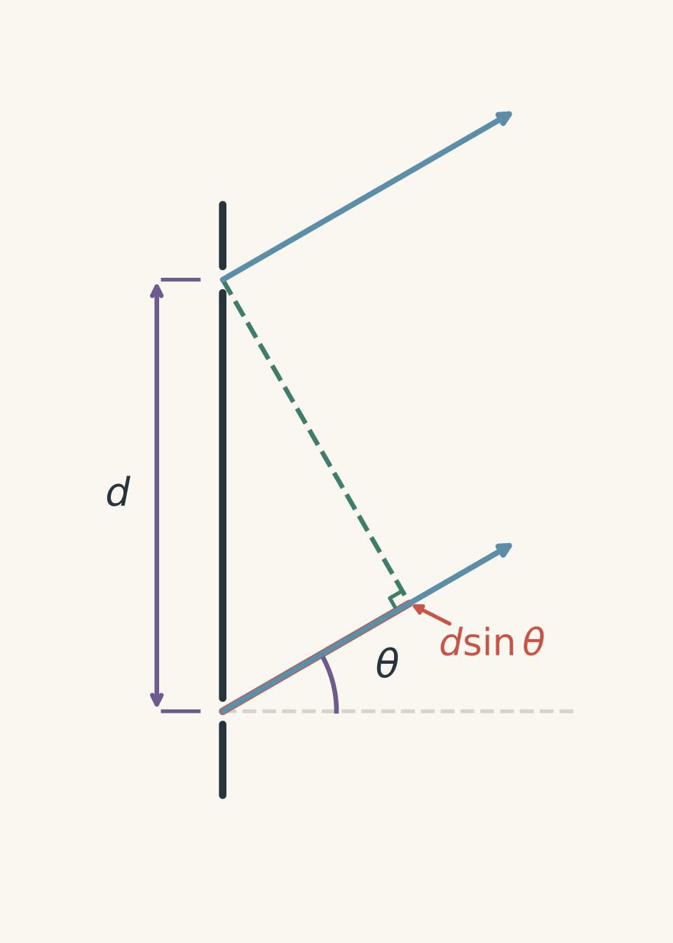
The extra distance travelled is
\[ d\sin\theta \]
where:
- \(d\) is the separation between neighbouring slits, in metres,
- \(\theta\) is the angle of the outgoing light measured from the normal to the grating.
Now make a prediction. When should the waves arrive in step and reinforce each other: when the extra path is half a wavelength, or a whole number of wavelengths?
A whole number. If the second wave travels exactly \(1\lambda\), \(2\lambda\), \(3\lambda\), and so on further than the first, a crest still arrives with a crest.
So the bright principal maxima satisfy
\[ d\sin\theta=m\lambda \]
where:
- \(\lambda\) is the wavelength of the light, in metres,
- \(m\) is the order of the maximum: \(0,\pm1,\pm2,\ldots\).
The central maximum has \(m=0\), so \(\theta=0^\circ\). First-order maxima have \(m=\pm1\), second-order maxima have \(m=\pm2\), and so on.
This is the same constructive-interference condition that appears with two slits. If that connection is rusty, the double-slit interference guide is a useful refresher.
A simple way to picture the grating is as a huge group trying to clap in time. At certain directions, the wave from every slit arrives “on the clap”, so the amplitudes add strongly. Move slightly away from that direction and the timing starts to drift across the group.
The analogy is useful for phase, but it has limits. The slits are not independent little objects deciding when to emit light. The grating is splitting one coherent wavefront, and the resulting wave amplitudes superpose.
02Converting lines per millimetre into slit spacing
Questions often give a grating as something like “500 lines per millimetre” rather than directly giving \(d\).
If the line density is \(n\), then
\[ d=\frac{1}{n} \]
provided \(n\) and \(d\) use matching units.
For example, \(500\) lines per millimetre means
\[ 500\text{ lines mm}^{-1} =500\,000\text{ lines m}^{-1}. \]
Therefore,
\[ d=\frac{1}{500\,000} =2.00\times10^{-6}\text{ m}. \]
One very common error is to use \(500\) directly in \(d=1/n\) and then treat the answer as metres. The unit conversion has to happen first.
Worked example: Find the diffraction angles and highest order
A diffraction grating has \(500\) lines per millimetre. Monochromatic light of wavelength \(600\text{ nm}\) is incident normally on the grating. Calculate the angles of the first three orders and determine whether a fourth-order maximum can exist.
Step 1
\[ n=500\times1000 =5.00\times10^5\text{ m}^{-1} \]
Step 2
\[ d=\frac{1}{n} =\frac{1}{5.00\times10^5} =2.00\times10^{-6}\text{ m} \]
The wavelength is
\[ \lambda=600\text{ nm} =6.00\times10^{-7}\text{ m}. \]
Step 3
For \(m=1\),
\[ \sin\theta =\frac{(1)(6.00\times10^{-7})}{2.00\times10^{-6}} =0.300 \]
so
\[ \theta=17.5^\circ. \]
Step 4
For \(m=2\),
\[ \sin\theta =\frac{2(6.00\times10^{-7})}{2.00\times10^{-6}} =0.600, \]
so
\[ \theta=36.9^\circ. \]
For \(m=3\),
\[ \sin\theta =\frac{3(6.00\times10^{-7})}{2.00\times10^{-6}} =0.900, \]
so
\[ \theta=64.2^\circ. \]
Step 5
For \(m=4\),
\[ \sin\theta =\frac{4(6.00\times10^{-7})}{2.00\times10^{-6}} =1.20. \]
But \(\sin\theta\) can never be greater than \(1\). Therefore, a fourth-order maximum cannot exist.
The grating produces first-, second-, and third-order maxima at \(17.5^\circ\), \(36.9^\circ\), and \(64.2^\circ\), respectively. The third order is the highest possible order.
03A quick way to find the highest possible order
Because
\[ \sin\theta\leq1, \]
the grating equation requires
\[ \frac{m\lambda}{d}\leq1. \]
Therefore,
\[ m\leq\frac{d}{\lambda}. \]
The largest allowed integer gives the highest possible order.
For the previous example,
\[ \frac{d}{\lambda} =\frac{2.00\times10^{-6}}{6.00\times10^{-7}} =3.33, \]
so the highest possible order is \(m=3\).
There is one practical detail worth knowing. If the calculation gives exactly \(\sin\theta=1\), then \(\theta=90^\circ\). That is mathematically allowed, but the light would travel parallel to the grating surface and would usually not be useful in a real spectrometer.
04Why a grating separates different wavelengths
Now imagine two wavelengths passing through the same grating.
For a fixed order \(m\),
\[ d\sin\theta=m\lambda. \]
If \(\lambda\) increases while \(d\) and \(m\) stay fixed, \(\sin\theta\) must increase. The longer wavelength therefore appears at a larger angle.
That is why a grating spreads white light into a spectrum. In a given order, red light appears at a larger angle from the centre than violet light.
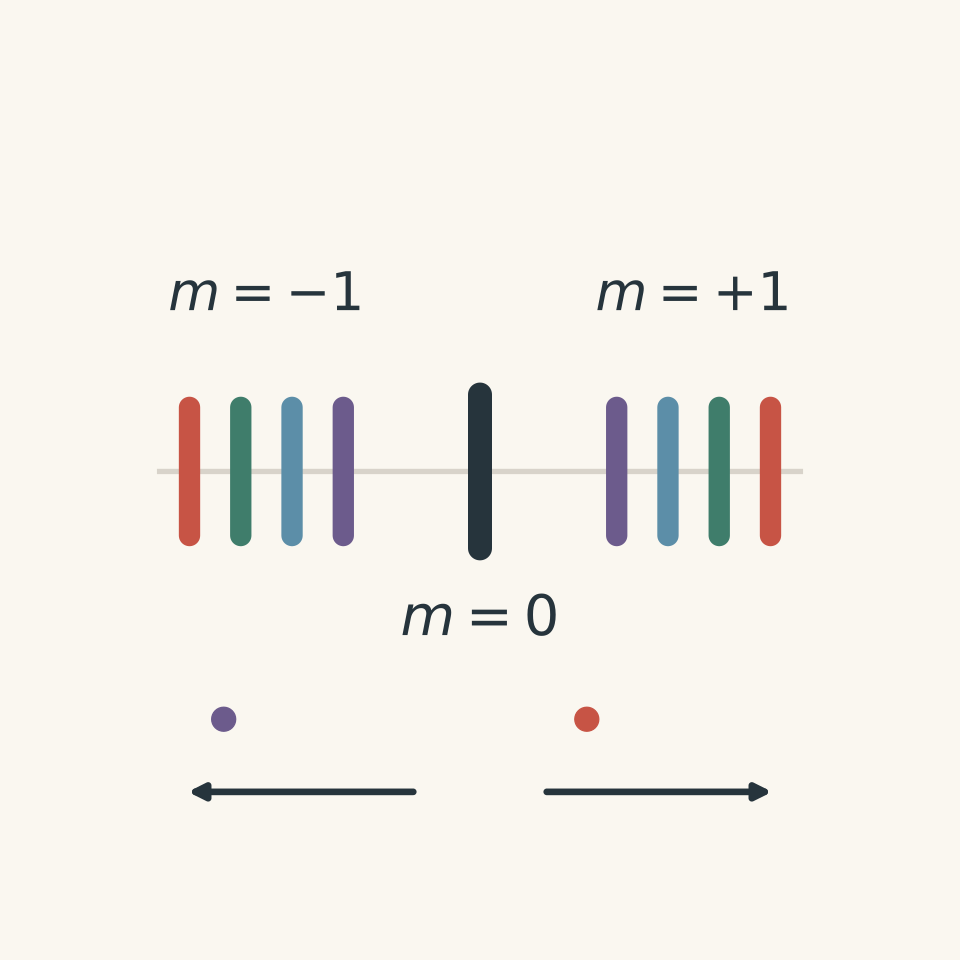
Notice something unusual about \(m=0\):
\[ d\sin0^\circ=0. \]
Every wavelength satisfies the condition there. So the central maximum does not separate wavelengths. Spectral separation begins in the non-zero orders.
For two nearby wavelengths, a useful approximation is
\[ \Delta\theta\approx \frac{m\Delta\lambda}{d\cos\theta}, \]
where \(\Delta\lambda\) is their wavelength difference and \(\Delta\theta\) is their small angular separation in radians.
This tells us that nearby wavelengths are generally separated more strongly when:
- the order \(m\) is larger,
- the slit spacing \(d\) is smaller,
- the diffraction angle is larger.
A smaller \(d\) means more grating lines per millimetre.
But angular separation is only half the story.
05Separation is not the same as resolution
Imagine two spectral lines whose maxima occur \(0.05^\circ\) apart.
That sounds promising. But what if each bright peak is \(0.10^\circ\) wide? They would overlap badly and probably look like one line.
Now imagine the same two maxima are \(0.05^\circ\) apart, but each peak is extremely narrow. The two lines can be distinguished.
That distinction is resolution.
A diffraction grating improves wavelength resolution because many equally spaced slits create much narrower principal maxima than a two-slit arrangement.
Why?
At the exact principal maximum, the waves from every slit arrive in phase. Move a little away from that angle and a small phase difference appears between neighbouring slits.
With only two slits, that small mismatch does not immediately destroy the bright fringe.
With hundreds or thousands of slits, the mismatch accumulates across the whole grating. Waves from different parts of the grating then cancel strongly. The intensity drops rapidly on either side of the exact maximum.
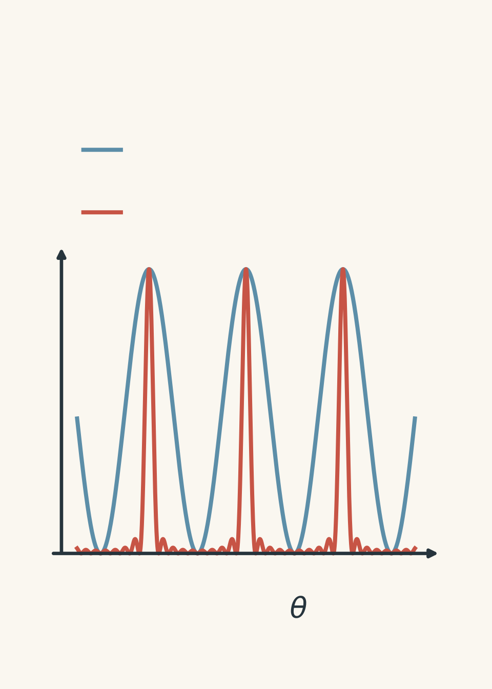
This gives an important distinction:
| Change | Main effect |
|---|---|
| Decrease \(d\), meaning more lines per millimetre | Usually increases angular separation of wavelengths |
| Increase the number of illuminated slits \(N\) | Makes principal maxima narrower |
| Increase diffraction order \(m\) | Increases both spectral dispersion and ideal resolving power |
The single-slit diffraction pattern still matters because each slit has a finite width. It creates an overall diffraction envelope that affects the intensities of the grating maxima. The diffraction of light guide explains that part in more detail.
06Resolving power of an ideal diffraction grating
For an ideal grating, its resolving power can be written as
\[ R=\frac{\lambda}{\Delta\lambda_{\min}}=mN \]
where:
- \(R\) is the resolving power,
- \(\lambda\) is the wavelength being observed,
- \(\Delta\lambda_{\min}\) is the smallest wavelength difference that can just be resolved,
- \(m\) is the diffraction order,
- \(N\) is the number of illuminated grating lines.
Therefore,
\[ \Delta\lambda_{\min} =\frac{\lambda}{mN}. \]
A larger value of \(mN\) means better wavelength resolution.
Do not confuse \(N\), the total number of illuminated lines, with the line density.
If a grating has line density \(n\) and an illuminated width \(W\), then approximately
\[ N=nW, \]
provided the units are consistent.
For example, a grating with \(600\) lines per millimetre illuminated across \(4.0\text{ mm}\) has
\[ N=(600)(4.0)=2400 \]
illuminated lines.
This resolving-power expression describes an ideal grating. A real spectrometer can also be limited by the entrance slit, detector resolution, optical aberrations, alignment, and other effects.
Worked example: Can two close wavelengths be resolved?
A grating has \(600\) lines per millimetre, and a \(4.0\text{ mm}\) width of the grating is illuminated. Two spectral lines have wavelengths \(589.0\text{ nm}\) and \(589.6\text{ nm}\). Determine whether they can ideally be resolved in second order.
Step 1
\[ N=(600\text{ lines mm}^{-1})(4.0\text{ mm}) =2400 \]
Step 2
Here \(m=2\), so
\[ R=mN=(2)(2400)=4800. \]
Step 3
Using a representative wavelength of about \(589.3\text{ nm}\),
\[ \Delta\lambda_{\min} =\frac{\lambda}{R} =\frac{589.3\text{ nm}}{4800} =0.123\text{ nm}. \]
Step 4
\[ \Delta\lambda =589.6-589.0 =0.600\text{ nm}. \]
Since
\[ 0.600\text{ nm}>0.123\text{ nm}, \]
the two lines can ideally be resolved.
The important point is not merely that their maxima occur at slightly different angles. The grating has enough illuminated lines, in a high enough order, to make the peaks narrow enough that the two wavelengths remain distinguishable.
07Don’t assume that more lines per millimetre always means “better”
This is the tempting shortcut.
A higher line density means a smaller spacing \(d\). From
\[ d\sin\theta=m\lambda, \]
that often produces a larger diffraction angle and greater angular separation between nearby wavelengths in the same order.
So far, so good.
But a smaller \(d\) also restricts the available orders because
\[ m\lambda\leq d. \]
A very high-density grating may therefore lose its second, third, or higher orders entirely.
That matters because resolving power is
\[ R=mN. \]
A lower-density grating may contain fewer illuminated lines but allow a much higher diffraction order. In some situations, it can equal or even exceed the resolving power of a denser grating.
So the correct question is not “Which grating has more lines per millimetre?”
It is “What combination of order and illuminated lines is actually available?”
08Other traps worth checking
A grating question often becomes much easier once you identify what each quantity controls.
| If you need to find… | Start with… |
|---|---|
| Slit spacing from line density | \(d=1/n\) |
| Angle of a spectral maximum | \(d\sin\theta=m\lambda\) |
| Highest possible order | \(m\leq d/\lambda\) |
| Number of illuminated lines | \(N=nW\) |
| Ideal resolving power | \(R=mN\) |
| Minimum resolvable wavelength difference | \(\Delta\lambda_{\min}=\lambda/(mN)\) |
Also watch for these misconceptions.
The diffraction angle does not increase directly in proportion to the order. What increases proportionally is \(\sin\theta\):
\[ \sin\theta=\frac{m\lambda}{d}. \]
So doubling \(m\) does not usually double \(\theta\).
The grating spacing \(d\) is also not the width of an individual slit. The spacing determines the locations of the interference maxima. The individual slit width helps determine the diffraction envelope.
Finally, if a screen is involved, geometry matters. If the screen is a perpendicular distance \(L\) from the grating and a maximum is displaced by \(x\) from the centre, then
\[ x=L\tan\theta. \]
Do not replace \(\tan\theta\) with \(\sin\theta\) unless a justified small-angle approximation is being used.
09Questions and solutions
Question 1
A diffraction grating has \(400\) lines per millimetre. Light of wavelength \(500\text{ nm}\) is incident normally on the grating.
Calculate the angle of the first-order maximum.
Solution 1
The first-order maximum occurs at approximately \(11.5^\circ\) from the normal.
First convert the line density:
\[ n=400\times1000 =4.00\times10^5\text{ m}^{-1}. \]
Therefore,
\[ d=\frac{1}{n} =\frac{1}{4.00\times10^5} =2.50\times10^{-6}\text{ m}. \]
For first order, \(m=1\), and
\[ \lambda=500\text{ nm} =5.00\times10^{-7}\text{ m}. \]
Using
\[ d\sin\theta=m\lambda, \]
we get
\[ \sin\theta =\frac{(1)(5.00\times10^{-7})}{2.50\times10^{-6}} =0.200. \]
Therefore,
\[ \theta=\sin^{-1}(0.200)=11.5^\circ. \]
The common trap is to treat \(400\text{ lines mm}^{-1}\) as \(400\text{ m}^{-1}\). Converting the line density before calculating \(d\) avoids that error.
Question 2
A grating has \(600\) lines per millimetre. It is illuminated with light containing wavelengths \(450\text{ nm}\) and \(650\text{ nm}\).
A detector can collect light only for diffraction angles up to \(50^\circ\) on either side of the centre.
For each wavelength, determine which non-zero diffraction orders are actually recorded.
Solution 2
The detector records first- and second-order maxima for \(450\text{ nm}\), but only the first-order maximum for \(650\text{ nm}\).
First find the grating spacing:
\[ n=600\times1000 =6.00\times10^5\text{ m}^{-1}, \]
so
\[ d=\frac{1}{6.00\times10^5} =1.667\times10^{-6}\text{ m}. \]
For \(450\text{ nm}\), the first order is
\[ \sin\theta_1 =\frac{450\times10^{-9}}{1.667\times10^{-6}} =0.270, \]
giving
\[ \theta_1=15.7^\circ. \]
The second order gives
\[ \sin\theta_2 =\frac{2(450\times10^{-9})}{1.667\times10^{-6}} =0.540, \]
so
\[ \theta_2=32.7^\circ. \]
The third order gives
\[ \sin\theta_3 =\frac{3(450\times10^{-9})}{1.667\times10^{-6}} =0.810, \]
so
\[ \theta_3=54.1^\circ. \]
The third-order maximum physically exists, but it lies outside the detector’s \(50^\circ\) range. The detector therefore records only \(m=1\) and \(m=2\) for \(450\text{ nm}\).
For \(650\text{ nm}\),
\[ \sin\theta_1 =\frac{650\times10^{-9}}{1.667\times10^{-6}} =0.390, \]
so
\[ \theta_1=23.0^\circ. \]
For second order,
\[ \sin\theta_2 =\frac{2(650\times10^{-9})}{1.667\times10^{-6}} =0.780, \]
which gives
\[ \theta_2=51.3^\circ. \]
That maximum also exists, but it falls just beyond the detector limit.
The tempting mistake is to ask only whether an order is mathematically possible. An order can satisfy \(\sin\theta\leq1\) and still be missed because the apparatus cannot collect light at that angle.
Question 3
A grating produces a first-order maximum for \(520\text{ nm}\) light at \(20.0^\circ\).
Determine:
- the grating spacing,
- the line density in lines per millimetre,
- the first-order angle for \(650\text{ nm}\) light,
- the angle of the second-order maximum for \(520\text{ nm}\).
A student claims that the last answer must be \(40.0^\circ\), because the order has doubled. Explain the error.
Solution 3
The grating spacing is \(1.52\times10^{-6}\text{ m}\), the line density is about \(658\text{ lines mm}^{-1}\), the \(650\text{ nm}\) first-order maximum is at about \(25.3^\circ\), and the \(520\text{ nm}\) second-order maximum is at about \(43.2^\circ\), not \(40.0^\circ\).
For the known first-order maximum,
\[ d\sin20.0^\circ=(1)(520\times10^{-9}\text{ m}). \]
Therefore,
\[ d =\frac{520\times10^{-9}}{\sin20.0^\circ} =1.52\times10^{-6}\text{ m}. \]
The line density is
\[ n=\frac{1}{d} =\frac{1}{1.52\times10^{-6}} \approx6.58\times10^5\text{ m}^{-1}. \]
Since \(1000\text{ mm}=1\text{ m}\),
\[ n\approx658\text{ lines mm}^{-1}. \]
For \(650\text{ nm}\) in first order,
\[ \sin\theta =\frac{650\times10^{-9}}{1.52\times10^{-6}} \approx0.428, \]
so
\[ \theta\approx25.3^\circ. \]
For \(520\text{ nm}\) in second order,
\[ \sin\theta =\frac{2(520\times10^{-9})}{1.52\times10^{-6}} \approx0.684, \]
giving
\[ \theta\approx43.2^\circ. \]
The student’s prediction feels reasonable because \(m\) appears directly in the grating equation. However, the equation says
\[ \sin\theta\propto m, \]
not
\[ \theta\propto m. \]
Doubling the order doubles \(\sin\theta\), not the angle itself. The nonlinear relationship between \(\theta\) and \(\sin\theta\) is what changes the result.
Question 4
Two gratings are available for separating spectral lines near \(500\text{ nm}\).
Grating A has \(600\) lines per millimetre.
Grating B has \(1200\) lines per millimetre.
In each case, \(2.0\text{ mm}\) of the grating is illuminated. A spectrometer can collect any maximum with \(\theta<80^\circ\).
Two spectral lines have wavelengths \(500.00\text{ nm}\) and \(500.18\text{ nm}\).
For each grating:
- determine the highest usable diffraction order,
- calculate the ideal resolving power in that order,
- decide whether the two wavelengths can be resolved.
Explain why simply choosing the grating with the greater line density gives the wrong conclusion.
Solution 4
Grating A can ideally resolve the two wavelengths in third order, while Grating B cannot resolve them at its highest available order. The lower-density grating performs better here because its extra available diffraction order more than compensates for its smaller number of illuminated lines.
For Grating A,
\[ n_A=600\text{ lines mm}^{-1}, \]
so
\[ d_A=\frac{1}{600\,000} =1.667\times10^{-6}\text{ m}. \]
The highest possible order near \(500\text{ nm}\) satisfies
\[ m\leq\frac{d_A}{\lambda} =\frac{1.667\times10^{-6}}{500\times10^{-9}} =3.33. \]
So the highest order is \(m=3\).
Check that the apparatus can collect it:
\[ \sin\theta =\frac{3(500\times10^{-9})}{1.667\times10^{-6}} =0.900, \]
so
\[ \theta=64.2^\circ, \]
which is below \(80^\circ\).
The number of illuminated lines is
\[ N_A=(600)(2.0)=1200. \]
Therefore,
\[ R_A=mN=(3)(1200)=3600. \]
The minimum resolvable wavelength difference is approximately
\[ \Delta\lambda_{\min,A} =\frac{500\text{ nm}}{3600} =0.139\text{ nm}. \]
Since
\[ 0.180\text{ nm}>0.139\text{ nm}, \]
Grating A can ideally resolve the pair.
For Grating B,
\[ d_B =\frac{1}{1.20\times10^6} =8.33\times10^{-7}\text{ m}. \]
The allowed order satisfies
\[ m\leq \frac{8.33\times10^{-7}}{500\times10^{-9}} =1.67. \]
So only \(m=1\) is available.
The illuminated number of lines is
\[ N_B=(1200)(2.0)=2400. \]
Hence
\[ R_B=(1)(2400)=2400. \]
Its minimum resolvable wavelength difference is
\[ \Delta\lambda_{\min,B} =\frac{500\text{ nm}}{2400} =0.208\text{ nm}. \]
Since
\[ 0.180\text{ nm}<0.208\text{ nm}, \]
Grating B cannot ideally resolve the two wavelengths.
The tempting route is to notice that Grating B has twice as many lines per millimetre and therefore twice as many illuminated lines. That is true, but incomplete.
Its smaller slit spacing removes the second and third orders. Because resolving power depends on the product \(mN\), Grating A’s third order gives
\[ 3\times1200=3600, \]
whereas Grating B can achieve only
\[ 1\times2400=2400. \]
The diffraction order is not a minor detail. It changes the result.
Question 5
Three gratings are illuminated across the same width of \(10.0\text{ mm}\). They are being considered for resolving two spectral lines near \(480\text{ nm}\) that are separated by \(0.030\text{ nm}\).
- Grating A: \(500\) lines per millimetre
- Grating B: \(1000\) lines per millimetre
- Grating C: \(1250\) lines per millimetre
Assume an ideal grating and that the highest physically allowed non-zero order can be used.
For each grating, determine the highest allowed order and maximum ideal resolving power. Decide which gratings can resolve the two lines.
Then use \(d\sin\theta=m\lambda\) and \(R=mN\) to explain why increasing the line density does not guarantee an increase in the maximum possible resolving power when the illuminated width is fixed.
Solution 5
Gratings A and B have the same maximum ideal resolving power of \(20\,000\) and can resolve the \(0.030\text{ nm}\) separation, while Grating C has a lower maximum resolving power of \(12\,500\) and cannot. The key constraint is that increasing line density increases \(N\) but can simultaneously force the highest usable order \(m\) to decrease.
For Grating A,
\[ d_A =\frac{1}{500\,000} =2.00\times10^{-6}\text{ m}. \]
At \(\lambda=480\text{ nm}\),
\[ m\leq \frac{2.00\times10^{-6}}{480\times10^{-9}} =4.17. \]
Therefore,
\[ m_{\max,A}=4. \]
The number of illuminated lines is
\[ N_A=(500)(10.0)=5000. \]
So
\[ R_{\max,A}=mN=(4)(5000)=20\,000. \]
Hence
\[ \Delta\lambda_{\min,A} =\frac{480\text{ nm}}{20\,000} =0.0240\text{ nm}. \]
Since \(0.030\text{ nm}>0.0240\text{ nm}\), Grating A can ideally resolve the lines.
For Grating B,
\[ d_B =\frac{1}{1.00\times10^6} =1.00\times10^{-6}\text{ m}. \]
Thus,
\[ m\leq \frac{1.00\times10^{-6}}{480\times10^{-9}} =2.08, \]
so
\[ m_{\max,B}=2. \]
The illuminated number of lines is
\[ N_B=(1000)(10.0)=10\,000. \]
Therefore,
\[ R_{\max,B} =(2)(10\,000) =20\,000. \]
Again,
\[ \Delta\lambda_{\min,B} =\frac{480\text{ nm}}{20\,000} =0.0240\text{ nm}. \]
So Grating B also resolves the \(0.030\text{ nm}\) separation.
For Grating C,
\[ d_C =\frac{1}{1.25\times10^6} =8.00\times10^{-7}\text{ m}. \]
The order must satisfy
\[ m\leq \frac{8.00\times10^{-7}}{480\times10^{-9}} =1.67. \]
Therefore,
\[ m_{\max,C}=1. \]
The number of illuminated lines is
\[ N_C=(1250)(10.0)=12\,500. \]
Its maximum ideal resolving power is
\[ R_{\max,C} =(1)(12\,500) =12\,500. \]
Therefore,
\[ \Delta\lambda_{\min,C} =\frac{480\text{ nm}}{12\,500} =0.0384\text{ nm}. \]
Because
\[ 0.030\text{ nm}<0.0384\text{ nm}, \]
Grating C cannot ideally resolve the pair.
The deeper result comes from combining the two governing constraints.
For any possible order,
\[ m\lambda\leq d, \]
so
\[ m\leq\frac{d}{\lambda}. \]
If the illuminated grating width is \(W\), then the number of illuminated lines is approximately
\[ N=\frac{W}{d}. \]
Since
\[ R=mN, \]
the maximum possible value is bounded by
\[ R \leq \frac{d}{\lambda}\frac{W}{d} =\frac{W}{\lambda}. \]
The spacing \(d\) cancels.
That is the hinge. Packing more lines into the same width raises \(N\), but the smaller spacing also reduces the orders that can exist. In an idealised continuous argument, those effects can cancel. In a real grating, \(m\) must be an integer, so the achievable resolving power changes in steps.
That explains the initially strange result. Grating B has twice the line density of A, but it has half the highest order, so their products \(mN\) are identical:
\[ (4)(5000)=(2)(10\,000)=20\,000. \]
Grating C pushes the density higher again, but its second order is no longer physically possible. Its extra illuminated lines are not enough to replace the lost order.
10What this lets you understand next
The grating equation tells you where each wavelength goes. Resolving power tells you whether two nearby wavelengths remain distinguishable once they get there.
The next useful step is to connect that behaviour back to ordinary interference and diffraction. A grating’s sharp principal maxima come from many-slit interference, while their overall brightness is controlled partly by the diffraction pattern from each individual slit. Together, those ideas explain not only where a spectrum appears, but why some orders can be strong, weak, or even effectively missing.