
Faraday’s Law for HSC Physics: Calculating Induced EMF
Learn how to calculate induced emf from changes in magnetic flux linkage using Faraday’s law, with worked examples and challenging HSC-style questions.
Suppose a coil sits in a magnetic field, and the field strength doubles. You might predict that the induced emf must increase. But what if the coil rotates at the same time, so that less of the field passes through it?
Make a prediction before going further: does a changing magnetic field automatically produce an induced emf?
No. Faraday’s law does not respond to magnetic field strength by itself. It responds to the rate of change of magnetic flux linkage. If one change increases the flux while another decreases it by exactly the same amount, the induced emf can be zero.
That is the calculation Faraday’s law gives us:
\[ \mathcal{E}=-\frac{\Delta(N\Phi)}{\Delta t} \]
The important part is understanding what \(N\Phi\) means, what can change it, and what the minus sign is telling you.
01What is actually changing?
Picture a single loop of wire sitting in a magnetic field. Some of the magnetic field passes through the area enclosed by the loop.
A useful mental model is a hoop held in falling rain. Turn the hoop face-on to the rain, and lots of rain passes through it. Turn it edge-on, and almost none does. A larger hoop also catches more rain.
For a magnetic field, the equivalent quantity is magnetic flux, \(\Phi\). It measures how much of the magnetic field passes through one loop.
The analogy has a limit. Magnetic field lines are not physical strands flowing through the coil, and magnetic flux is not a substance that gets trapped inside it. The picture is only helping us think about area and orientation.
Now suppose the wire has 100 turns rather than one. Each turn has the same magnetic flux through it, so the effect is multiplied by 100. This gives the magnetic flux linkage:
\[ \lambda=N\Phi \]
where:
- \(\lambda\) is magnetic flux linkage, commonly described in weber-turns,
- \(N\) is the number of turns in the coil, and
- \(\Phi\) is the magnetic flux through one turn, measured in webers, \(\text{Wb}\).
Faraday’s law cares about how quickly this flux linkage changes.
02Magnetic flux comes before Faraday’s law
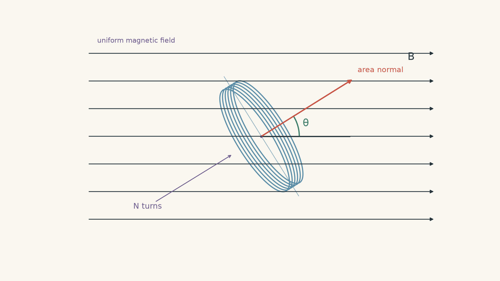
For a uniform magnetic field passing through a flat coil,
\[ \Phi=BA\cos\theta \]
where \(B\) is magnetic field strength in teslas, \(\text{T}\), \(A\) is the area of one loop in square metres, \(\text{m}^2\), and \(\theta\) is the angle between the magnetic field and the line perpendicular to the plane of the coil.
That last phrase causes a lot of errors. The angle is measured from the normal to the coil, not from the surface of the coil.
| Position of the coil | Angle \(\theta\) between \(B\) and the normal | Magnetic flux |
|---|---|---|
| Plane of coil perpendicular to field | \(0^\circ\) | Maximum: \(\Phi=BA\) |
| Plane of coil tilted | Between \(0^\circ\) and \(90^\circ\) | Between \(0\) and \(BA\) |
| Plane of coil parallel to field | \(90^\circ\) | Zero |
If this geometry still feels slippery, revise magnetic flux and \(\Phi=BA\cos\theta\) before pushing further.
Because
\[ N\Phi=NBA\cos\theta, \]
flux linkage can change because \(B\), \(A\), or \(\theta\) changes. Faraday’s law does not care which one caused the change.
03Faraday’s law turns flux change into emf
For a fixed number of turns,
\[ \mathcal{E}_{\text{avg}} =-N\frac{\Delta\Phi}{\Delta t} \]
or, equivalently,
\[ \mathcal{E}_{\text{avg}} =-\frac{\Delta(N\Phi)}{\Delta t}. \]
Here, \(\mathcal{E}_{\text{avg}}\) is the average induced emf in volts, \(\text{V}\), and \(\Delta t\) is the time interval in seconds, \(\text{s}\).
The magnitude is
\[ |\mathcal{E}_{\text{avg}}| =\frac{|\Delta(N\Phi)|}{\Delta t}. \]
This is basically a speed calculation. Speed tells you how quickly position changes. Faraday’s law tells you how quickly flux linkage changes.
A flux-linkage change of \(3.0\ \text{Wb-turn}\) in \(1.0\ \text{s}\) gives an average emf magnitude of \(3.0\ \text{V}\). A change of the same size in \(0.10\ \text{s}\) gives \(30\ \text{V}\).
Same change. Less time. Larger rate of change.
The unit relationship is useful:
\[ 1\ \text{V}=1\ \text{Wb s}^{-1}. \]
04What does the minus sign mean?
Suppose positive magnetic flux through a coil is increasing. Faraday’s law gives a negative emf relative to the positive direction you chose around the circuit.
The minus sign is Lenz’s law in mathematical form. The induced effect opposes the change in flux, not necessarily the magnetic field itself.
If positive flux is increasing, the induced current creates a magnetic field that tends to oppose that increase.
If positive flux is decreasing, the induced current creates a magnetic field that tends to maintain it.
This is why it is usually safest to calculate the magnitude first, then reason separately about direction when the question asks for it.
Worked example: a magnetic field gets stronger
An 80-turn coil has an area of \(1.5\times10^{-2}\ \text{m}^2\). Its area normal is parallel to a uniform magnetic field. The field increases from \(0.20\ \text{T}\) to \(0.55\ \text{T}\) in \(0.30\ \text{s}\). Calculate the magnitude of the average induced emf.
Step 1
The area and orientation stay constant. Only \(B\) changes. Because \(\theta=0^\circ\),
\[ \Phi=BA. \]
So the change in flux through one turn is
\[ \Delta\Phi =A(B_f-B_i) =(1.5\times10^{-2})(0.55-0.20) =5.25\times10^{-3}\ \text{Wb}. \]
Step 2
There are 80 turns:
\[ \Delta(N\Phi) =N\Delta\Phi =80(5.25\times10^{-3}) =0.420\ \text{Wb-turn}. \]
Step 3
\[ |\mathcal{E}_{\text{avg}}| =\frac{0.420}{0.30} =1.40\ \text{V}. \]
The average induced emf has a magnitude of \(1.40\ \text{V}\). Because the original flux is increasing, the induced effect acts in a direction that opposes that increase.
Notice that the final magnetic field strength, \(0.55\ \text{T}\), is not enough by itself to determine the emf. We needed the change in flux and the time taken.
05A reliable calculation method
When you see a Faraday’s law calculation, use the same sequence each time:
- Work out what changes: \(B\), \(A\), \(\theta\), or some combination of them.
- Calculate the initial and final flux using \(\Phi=BA\cos\theta\). Check whether the stated angle is measured from the coil or from its normal.
- Find the change in flux linkage, \(\Delta(N\Phi)=N(\Phi_f-\Phi_i)\).
- Divide by the time interval to obtain the average emf.
- If direction is required, use the minus sign and Lenz’s law to decide which change the induced effect must oppose.
This method is slightly longer than trying to spot a shortcut, but it survives much harder questions.
Worked example: the coil rotates
A 150-turn coil has area \(2.0\times10^{-2}\ \text{m}^2\) and sits in a \(0.40\ \text{T}\) uniform magnetic field. The angle between the magnetic field and the coil’s area normal changes from \(30^\circ\) to \(75^\circ\) in \(0.120\ \text{s}\). Calculate the magnitude of the average induced emf.
Step 1
\[ \Phi_i =BA\cos\theta_i =(0.40)(2.0\times10^{-2})\cos30^\circ =6.93\times10^{-3}\ \text{Wb}. \]
Step 2
\[ \Phi_f =(0.40)(2.0\times10^{-2})\cos75^\circ =2.07\times10^{-3}\ \text{Wb}. \]
The flux has decreased because the coil has rotated towards an edge-on orientation.
Step 3
\[ \begin{aligned} \Delta(N\Phi) &=N(\Phi_f-\Phi_i)\\ &=150(2.07\times10^{-3}-6.93\times10^{-3})\\ &=-0.729\ \text{Wb-turn}. \end{aligned} \]
Step 4
\[ \begin{aligned} \mathcal{E}_{\text{avg}} &=-\frac{\Delta(N\Phi)}{\Delta t}\\ &=-\frac{-0.729}{0.120}\\ &=6.07\ \text{V}. \end{aligned} \]
The average induced emf has a magnitude of about \(6.1\ \text{V}\).
The positive sign here depends on the positive direction chosen for flux and emf. Physically, the useful conclusion is that the original positive flux is decreasing, so the induced effect acts to support that flux.
06The tempting misconception: changing \(B\) means induced emf
Imagine a coil sitting completely still in a steady \(5.0\ \text{T}\) magnetic field. Its flux may be large, but its flux linkage is not changing.
So:
\[ \Delta(N\Phi)=0 \]
and therefore
\[ \mathcal{E}=0. \]
A large magnetic flux is not enough. You need a change in magnetic flux linkage.
Now reverse the situation. Suppose the magnetic field strength stays perfectly constant, but the coil rotates. The angle \(\theta\) changes, so \(BA\cos\theta\) changes. An emf is induced even though \(B\) never changes.
There is an even sneakier possibility. Both \(B\) and \(\theta\) can change while the flux stays constant. For example, if \(B\) doubles while \(\cos\theta\) halves, then \(B\cos\theta\) is unchanged. If \(N\) and \(A\) are also constant, the flux linkage does not change, so no emf is induced.
Faraday’s law watches the whole product, not one variable in isolation.
07Average emf can hide what happened in between
For changes over a finite time interval,
\[ \mathcal{E}_{\text{avg}} =-\frac{\Delta(N\Phi)}{\Delta t}. \]
This tells you the average emf between the two endpoints.
If flux linkage changes at a constant rate, that average is also the emf throughout the interval.
But suppose the flux linkage rises for half a second and then falls back to its original value during the next half-second. Its total change over the full second is zero, so the average emf over that full second is zero.
That does not mean the emf was zero throughout the second.
At any particular instant, Faraday’s law can be written as
\[ \mathcal{E}=-\frac{d(N\Phi)}{dt}. \]
You do not need complicated calculus for most HSC questions. The important idea is that emf depends on the local rate of change. Positive and negative emfs can cancel when you calculate an average over a longer interval.
One more distinction matters. An induced emf can exist even if the circuit is open. A current only flows if there is a conducting path. Faraday’s law predicts the emf; the circuit’s resistance and connections determine the resulting current.
08Questions and solutions
Question 1
A 120-turn coil has a magnetic flux through each turn that decreases from \(4.5\times10^{-4}\ \text{Wb}\) to \(1.5\times10^{-4}\ \text{Wb}\) in \(2.0\times10^{-2}\ \text{s}\).
Calculate the magnitude of the average induced emf.
Solution 1
The average induced emf is \(1.8\ \text{V}\).
The flux change through each turn is
\[ \Delta\Phi =1.5\times10^{-4}-4.5\times10^{-4} =-3.0\times10^{-4}\ \text{Wb}. \]
Using Faraday’s law,
\[ \begin{aligned} |\mathcal{E}_{\text{avg}}| &=N\frac{|\Delta\Phi|}{\Delta t}\\ &=120\frac{3.0\times10^{-4}}{2.0\times10^{-2}}\\ &=1.8\ \text{V}. \end{aligned} \]
The tempting route is to divide the flux change through one turn by the time and stop there. That would ignore the other 119 turns. Faraday’s law uses the change in total flux linkage, so the per-turn change must be multiplied by \(N=120\).
Because the original flux is decreasing, the induced effect acts to oppose that decrease.
Question 2
A 250-turn coil has an area of \(3.2\times10^{-3}\ \text{m}^2\) and is in a uniform \(0.60\ \text{T}\) magnetic field.
Initially, the plane of the coil is perpendicular to the magnetic field. It then rotates so that the plane of the coil makes an angle of \(50^\circ\) with the magnetic field. The rotation takes \(0.080\ \text{s}\).
Calculate the magnitude of the average induced emf, and state what the induced magnetic field attempts to do to the original flux.
Solution 2
The average induced emf is approximately \(1.4\ \text{V}\), and the induced magnetic field acts to oppose the decrease in the original flux.
Initially, the plane is perpendicular to the field. The area normal is therefore parallel to the field:
\[ \theta_i=0^\circ. \]
At the end, the plane makes \(50^\circ\) with the field. The normal therefore makes
\[ \theta_f=90^\circ-50^\circ=40^\circ \]
with the field.
The initial and final fluxes through one turn are
\[ \begin{aligned} \Phi_i&=BA\cos0^\circ\\ &=(0.60)(3.2\times10^{-3})\\ &=1.92\times10^{-3}\ \text{Wb}, \end{aligned} \]
and
\[ \begin{aligned} \Phi_f &=(0.60)(3.2\times10^{-3})\cos40^\circ\\ &=1.47\times10^{-3}\ \text{Wb}. \end{aligned} \]
Therefore,
\[ \begin{aligned} |\mathcal{E}_{\text{avg}}| &=N\frac{|\Phi_f-\Phi_i|}{\Delta t}\\ &=250\frac{|1.47\times10^{-3}-1.92\times10^{-3}|}{0.080}\\ &\approx1.40\ \text{V}. \end{aligned} \]
The tempting mistake is to substitute \(50^\circ\) directly into \(BA\cos\theta\). The given \(50^\circ\) is measured from the plane of the coil, while \(\theta\) in the flux equation is measured from its normal.
The flux decreases during the rotation, so Lenz’s law says the induced magnetic field acts in a direction that tends to maintain the original flux.
Question 3
A 100-turn rectangular coil initially has an area of \(5.0\times10^{-3}\ \text{m}^2\). Its area normal remains parallel to the magnetic field.
During the first \(0.10\ \text{s}\), its area stays constant while the magnetic field increases uniformly from \(0.20\ \text{T}\) to \(0.50\ \text{T}\).
During the next \(0.20\ \text{s}\), the magnetic field remains at \(0.50\ \text{T}\), while the area enclosed by each turn decreases uniformly from \(5.0\times10^{-3}\ \text{m}^2\) to \(2.0\times10^{-3}\ \text{m}^2\).
Find the average induced emf during each stage and determine whether the induced emf has the same or opposite direction in the two stages.
Solution 3
The average emf magnitude is \(1.5\ \text{V}\) during the first stage and \(0.75\ \text{V}\) during the second, and the two emfs have opposite directions.
Because \(\theta=0^\circ\),
\[ \Phi=BA. \]
During the first stage, the area is constant:
\[ \begin{aligned} \Delta(N\Phi) &=NA(B_f-B_i)\\ &=100(5.0\times10^{-3})(0.50-0.20)\\ &=0.150\ \text{Wb-turn}. \end{aligned} \]
So
\[ \mathcal{E}_{1} =-\frac{0.150}{0.10} =-1.5\ \text{V}. \]
Its magnitude is \(1.5\ \text{V}\).
During the second stage, \(B=0.50\ \text{T}\) is constant, but the area changes:
\[ \begin{aligned} \Delta(N\Phi) &=NB(A_f-A_i)\\ &=100(0.50)(2.0\times10^{-3}-5.0\times10^{-3})\\ &=-0.150\ \text{Wb-turn}. \end{aligned} \]
Therefore,
\[ \mathcal{E}_{2} =-\frac{-0.150}{0.20} =+0.75\ \text{V}. \]
The signs are opposite because the flux linkage increases in the first stage but decreases in the second.
It is tempting to look only for a changing magnetic field and conclude that induction stops once \(B\) becomes constant. The constraint Faraday’s law actually imposes is on \(N\Phi=NBA\cos\theta\). Changing the loop area changes the flux even when the magnetic field itself does not change.
Question 4
A 200-turn coil has an area of \(1.0\times10^{-2}\ \text{m}^2\). Its initial magnetic flux linkage is
\[ \lambda_i=+0.50\ \text{Wb-turn}. \]
Using the sign convention
\[ \mathcal{E}=-\frac{d\lambda}{dt}, \]
a voltmeter records the following:
- \(+4.0\ \text{V}\) for \(0.10\ \text{s}\),
- \(0\ \text{V}\) for the next \(0.20\ \text{s}\),
- \(-1.0\ \text{V}\) for the next \(0.30\ \text{s}\).
Assume the emf is constant during each stated interval.
Determine the final flux linkage and the final value of \(B\cos\theta\). Does the zero-emf interval prove that neither the coil nor the magnetic field was changing? Also determine whether the flux linkage changed sign at any time.
Solution 4
The final flux linkage is \(+0.40\ \text{Wb-turn}\), the final value of \(B\cos\theta\) is \(0.20\ \text{T}\), the zero-emf interval does not prove that the physical conditions were stationary, and the flux linkage never changes sign.
For an interval with constant emf,
\[ \Delta\lambda=-\mathcal{E}\Delta t. \]
During the first interval,
\[ \Delta\lambda_1 =-(+4.0)(0.10) =-0.40\ \text{Wb-turn}. \]
So
\[ \lambda_1 =0.50-0.40 =+0.10\ \text{Wb-turn}. \]
During the zero-emf interval,
\[ \Delta\lambda_2=0, \]
so the flux linkage remains
\[ \lambda_2=+0.10\ \text{Wb-turn}. \]
During the final interval,
\[ \Delta\lambda_3 =-(-1.0)(0.30) =+0.30\ \text{Wb-turn}. \]
Therefore,
\[ \lambda_f =0.10+0.30 =+0.40\ \text{Wb-turn}. \]
Now
\[ \lambda=N\Phi=NBA\cos\theta. \]
Hence
\[ \begin{aligned} B\cos\theta &=\frac{\lambda_f}{NA}\\ &=\frac{0.40}{(200)(1.0\times10^{-2})}\\ &=0.20\ \text{T}. \end{aligned} \]
The zero-emf interval only tells us that the flux linkage was constant:
\[ \frac{d\lambda}{dt}=0. \]
It does not prove that \(B\), \(A\), and \(\theta\) were all individually constant. For example, \(B\) could increase while the coil rotated so that \(B\cos\theta\) remained unchanged.
The flux linkage falls from \(+0.50\) to \(+0.10\ \text{Wb-turn}\), remains there, and then rises to \(+0.40\ \text{Wb-turn}\). It therefore never reaches zero and never changes sign.
A tempting interpretation is that an emf reading directly reveals what the magnetic field itself is doing. It does not. The measurement constrains the rate of change of the combined quantity \(NBA\cos\theta\), so several different physical motions or field changes can produce the same emf data.
Question 5
Two experiments use the same 200-turn coil of area \(1.0\times10^{-2}\ \text{m}^2\), connected to a \(4.0\ \Omega\) resistor. Ignore all other resistance and self-inductance.
In both experiments, the initial conditions are
\[ B_i=0.20\ \text{T},\qquad \theta_i=0^\circ. \]
After \(0.20\ \text{s}\), the final conditions are
\[ B_f=0.40\ \text{T},\qquad \theta_f=60^\circ. \]
In experiment A, \(B\) and \(\theta\) are adjusted together so that \(B\cos\theta=0.20\ \text{T}\) at every instant.
In experiment B, the coil remains at \(\theta=0^\circ\) for the first \(0.10\ \text{s}\) while \(B\) increases from \(0.20\ \text{T}\) to \(0.40\ \text{T}\). During the next \(0.10\ \text{s}\), \(B\) remains at \(0.40\ \text{T}\) while the coil rotates to \(60^\circ\). Assume the flux linkage changes uniformly during each stage.
A student argues that the two experiments are electrically equivalent because they have the same initial and final flux linkage, so the induced emf is zero.
Evaluate the claim. Calculate the emf, current, and thermal energy dissipated in the resistor for each experiment.
Solution 5
The experiments are not electrically equivalent. Experiment A has zero induced emf, zero current, and zero thermal energy dissipation throughout. Experiment B has emfs of \(-4.0\ \text{V}\) and \(+4.0\ \text{V}\) in its two stages, currents of magnitude \(1.0\ \text{A}\) in opposite directions, and dissipates \(0.80\ \text{J}\) of thermal energy in total. Both experiments nevertheless have an average emf of zero over the complete \(0.20\ \text{s}\).
First calculate the initial flux linkage:
\[ \begin{aligned} \lambda_i &=NBA\cos\theta_i\\ &=(200)(0.20)(1.0\times10^{-2})\cos0^\circ\\ &=0.40\ \text{Wb-turn}. \end{aligned} \]
The final flux linkage is
\[ \begin{aligned} \lambda_f &=(200)(0.40)(1.0\times10^{-2})\cos60^\circ\\ &=0.40\ \text{Wb-turn}. \end{aligned} \]
So the total change between the beginning and end is indeed zero.
In experiment A, however, something stronger is true. We are told that
\[ B\cos\theta=0.20\ \text{T} \]
at every instant. Since \(N\) and \(A\) are constant,
\[ \lambda=NBA\cos\theta \]
is constant at every instant.
Therefore,
\[ \mathcal{E}=0, \qquad I=\frac{\mathcal{E}}{R}=0. \]
With no current,
\[ E_{\text{thermal}}=0. \]
Now consider experiment B.
During the first stage, \(\theta=0^\circ\), so the flux linkage increases from
\[ 0.40\ \text{Wb-turn} \]
to
\[ \lambda =(200)(0.40)(1.0\times10^{-2}) =0.80\ \text{Wb-turn}. \]
Thus,
\[ \begin{aligned} \mathcal{E}_1 &=-\frac{0.80-0.40}{0.10}\\ &=-4.0\ \text{V}. \end{aligned} \]
The current is
\[ I_1=\frac{-4.0}{4.0}=-1.0\ \text{A}. \]
During the second stage, the flux linkage falls from \(0.80\) back to \(0.40\ \text{Wb-turn}\):
\[ \begin{aligned} \mathcal{E}_2 &=-\frac{0.40-0.80}{0.10}\\ &=+4.0\ \text{V}. \end{aligned} \]
Therefore,
\[ I_2=\frac{+4.0}{4.0}=+1.0\ \text{A}. \]
The current reverses direction because the direction of the flux-linkage change reverses.
The power dissipated in the resistor during either stage is
\[ P=I^2R=(1.0)^2(4.0)=4.0\ \text{W}. \]
This occurs for a total of \(0.20\ \text{s}\), so
\[ E_{\text{thermal}} =P\Delta t =(4.0)(0.20) =0.80\ \text{J}. \]
Why does this not contradict the zero overall change in flux linkage?
Over the whole interval,
\[ \mathcal{E}_{\text{avg}} =-\frac{\lambda_f-\lambda_i}{0.20} =0. \]
But that is a signed average. The \(-4.0\ \text{V}\) contribution from the first half cancels the \(+4.0\ \text{V}\) contribution from the second half.
Thermal energy does not cancel in the same way because resistive heating depends on \(I^2R\). A current of \(+1.0\ \text{A}\) and a current of \(-1.0\ \text{A}\) both heat the resistor.
The tempting route is to compare only the initial and final states and conclude that \(\Delta(N\Phi)=0\) means there was never an emf. The exact constraint is more subtle: zero total change guarantees only zero average emf over the complete interval. To know whether induction occurred during the interval, you need to know how the flux linkage changed with time.
That distinction is the bridge to generators. Once a coil rotates continuously, its flux linkage changes continuously too. Faraday’s law then lets you move from a changing \(BA\cos\theta\) to a changing induced emf, while Lenz’s law tells you the direction of the resulting current.