
Radioactive Half-Life: HSC Physics Calculations Explained
Learn how radioactive half-life works by modelling repeated halving, making quantitative predictions, and handling detector background readings and mixed isotopes.
Suppose a radioactive sample has a count rate of 1600 counts/min and a half-life of 6.0 h. What should you expect after 15 h?
It can’t be 800 counts/min, because that’s the value after one half-life. It also isn’t sensible to subtract the same number of counts every 6 h. The second interval removes half of what is left, not the same absolute amount as the first.
Before reading on, predict: after 15 h, should the count rate be above or below 400 counts/min?
It must be below 400 counts/min, because 15 h is more than two half-lives. The calculation gives about 283 counts/min.
That simple idea – keep halving what remains – is the core of radioactive half-life.
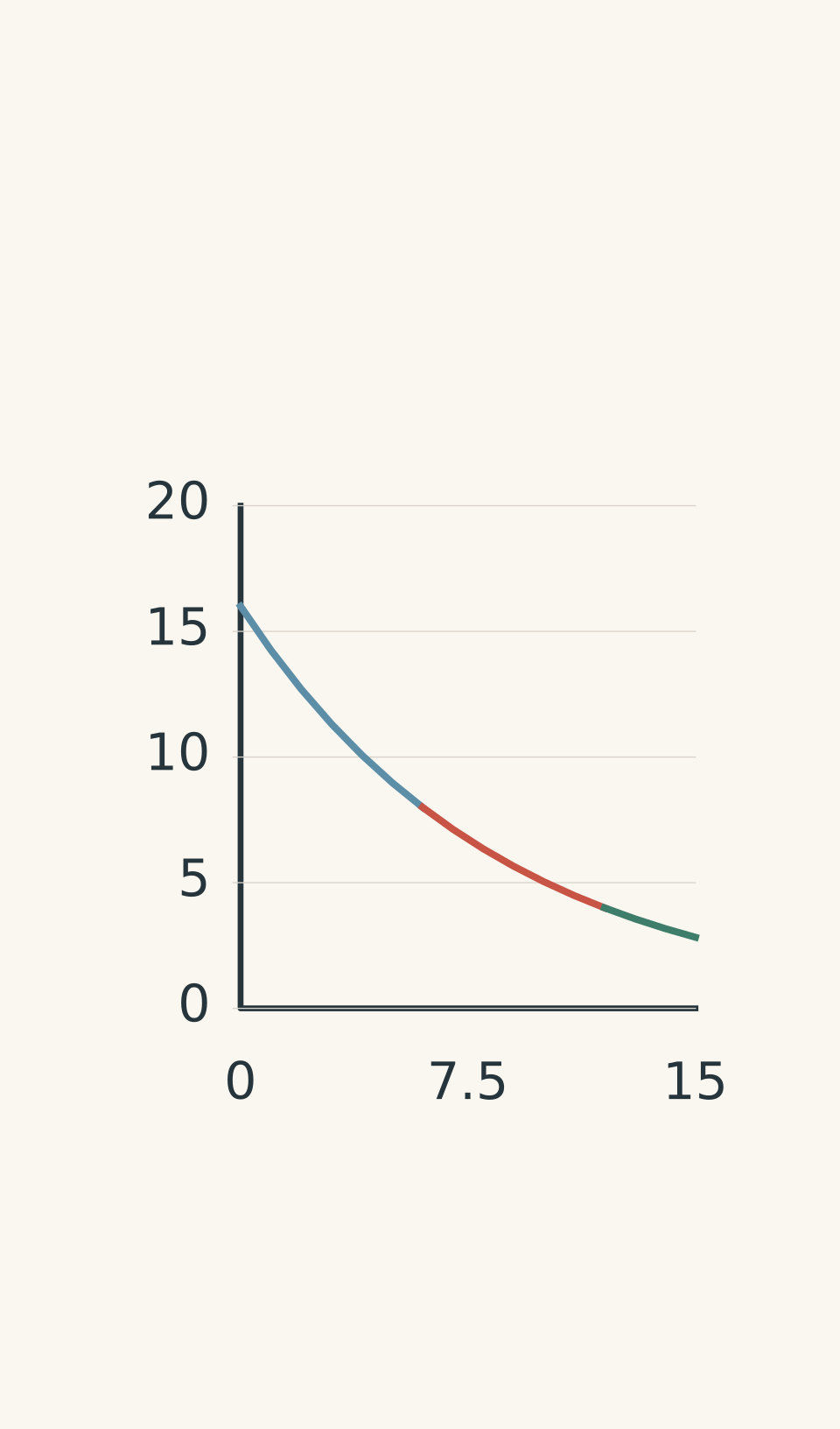
- 0–6 h: 1600 → 800
- 6–12 h: 800 → 400
- 12–15 h: 400 → ≈283
01See the halving before using the equation
Imagine a group of 1000 people in a club where, during each fixed interval, half of whoever is still there leaves.
After one interval, 500 remain.
After the next interval, half of those 500 leave, so 250 remain.
Then 125, then 62.5, and so on.
Radioactive decay follows this pattern statistically. The nuclei do not take turns in a neat queue. Each individual nucleus has a probability of decaying, and you cannot predict exactly which nucleus will decay next. For a large collection of nuclei, however, the number remaining follows a very predictable pattern.
The analogy breaks here: a radioactive sample does not literally send exactly half its nuclei away at the same instant. The half-life describes the statistical behaviour of the collection.
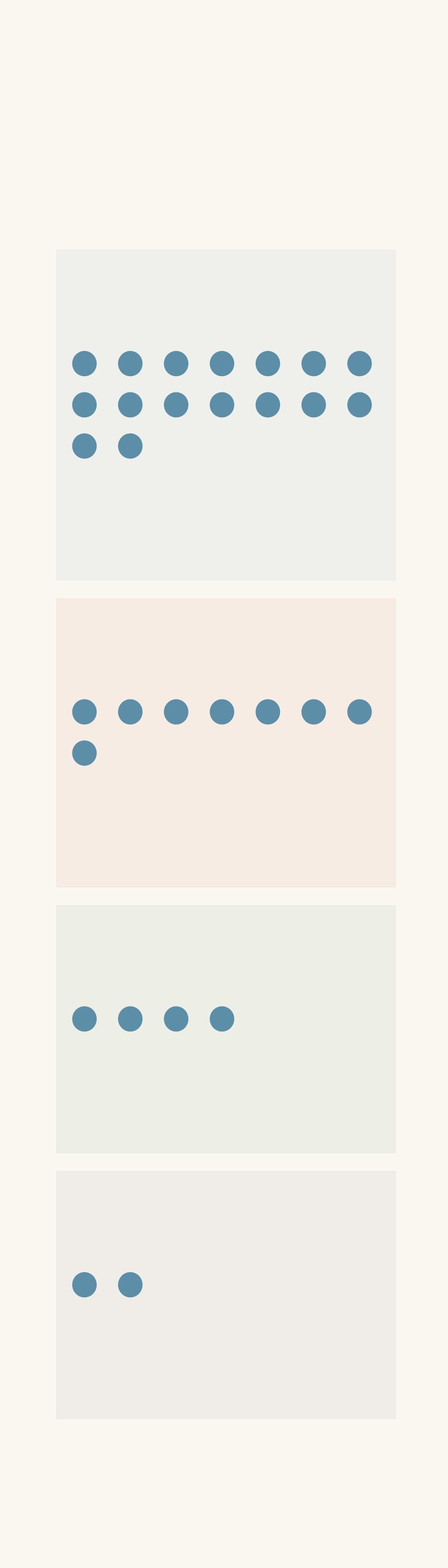
- Undecayed nuclei
So the important phrase is:
Half-life means half of what remains, not half of the original amount every time.
That is why the amount lost gets smaller:
- 1000 → 500: 500 disappear
- 500 → 250: 250 disappear
- 250 → 125: 125 disappear
The percentage change is the same. The absolute change is not.
02From repeated halving to a formula
For a single radioactive isotope, the half-life \(T_{1/2}\) is the time required for the number of undecayed nuclei to fall to half its value.
If \(n\) complete half-lives have passed, then
\[ N=N_0\left(\frac{1}{2}\right)^n \]
where:
- \(N_0\) is the initial number of undecayed nuclei,
- \(N\) is the number remaining,
- \(n\) is the number of half-lives that have passed.
Since
\[ n=\frac{t}{T_{1/2}} \]
we get
\[ N=N_0\left(\frac{1}{2}\right)^{t/T_{1/2}} \]
where \(t\) is the elapsed time.
This is an exponential relationship, not a linear one.
The same decay factor can be applied to the activity of a sample. Activity, measured in becquerels (Bq), is the number of nuclear decays per second. For one isotope, it follows the same half-life:
\[ A=A_0\left(\frac{1}{2}\right)^{t/T_{1/2}} \]
Here, \(A_0\) is the initial activity and \(A\) is the activity after time \(t\).
The radioactive isotope’s mass also follows the same pattern, provided you mean the mass of the radioactive parent isotope itself, rather than the total mass of everything in the container.
A useful half-life table
| Half-lives passed | Fraction remaining | Percentage remaining |
|---|---|---|
| 0 | \(1\) | 100% |
| 1 | \(1/2\) | 50% |
| 2 | \(1/4\) | 25% |
| 3 | \(1/8\) | 12.5% |
| 4 | \(1/16\) | 6.25% |
| 5 | \(1/32\) | 3.125% |
| 10 | \(1/1024\) | about 0.098% |
Notice that ten half-lives still does not give exactly zero. The amount gets very small, but the mathematical model approaches zero rather than reaching it after a fixed number of half-lives.
03What if the time is not a whole number of half-lives?
This is where the simple “halve it three times” method stops being enough.
Suppose the half-life is 8.0 h and the sample has been decaying for 20 h.
The number of half-lives is
\[ n=\frac{20}{8.0}=2.5 \]
So the remaining fraction is
\[ \left(\frac12\right)^{2.5}\approx0.177 \]
About 17.7% remains.
That may look strange at first. Half a half-life does not mean that another 25% of the original sample disappears. The decay is continuous, so for fractional half-lives you use the exponential equation rather than trying to invent another halving rule.
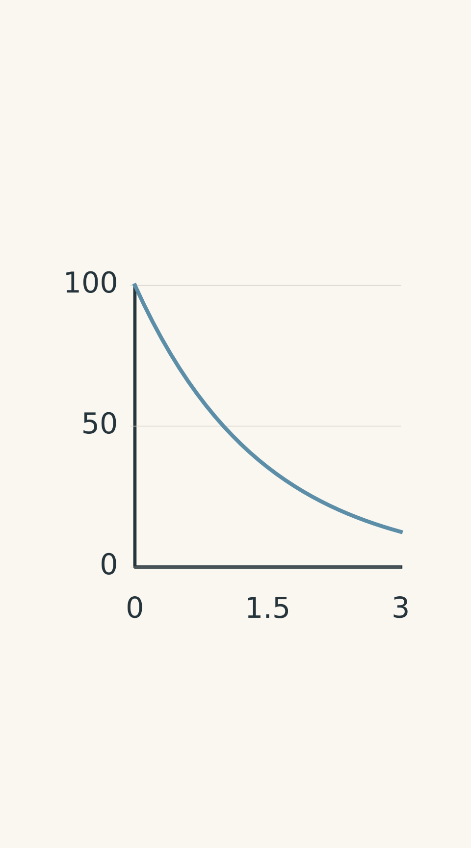
- Exponential decay
- 2.5 half-lives: 17.7% remains, not 0%
Worked example: Activity after three half-lives
A radioactive sample has an initial activity of 4800 Bq and a half-life of 2.0 h. What is its activity after 6.0 h?
Step 1
\[ n=\frac{t}{T_{1/2}} =\frac{6.0\text{ h}}{2.0\text{ h}} =3 \]
Three half-lives have passed.
Step 2
\[ A=A_0\left(\frac12\right)^n \]
\[ A=4800\left(\frac12\right)^3 \]
\[ A=600\text{ Bq} \]
Step 3
After 6.0 h, the activity is 600 Bq. The sample has gone through three halvings:
\[ 4800\rightarrow2400\rightarrow1200\rightarrow600 \]
Only \(1/8\), or 12.5%, of the original activity remains.
04Detector readings need one extra step
A detector does not necessarily record every decay from the sample. It measures a count rate, and there may also be radiation coming from the surroundings.
If the background is constant,
\[ C_{\text{measured}} = C_{\text{sample}} + C_{\text{background}} \]
where each \(C\) is a count rate, such as counts/min.
The half-life applies to the sample’s count rate, not to the background.
So if a detector reads 700 counts/min and the background is 100 counts/min, the radioactive sample is contributing only
\[ 700-100=600\text{ counts/min} \]
You halve that 600, not the 700.
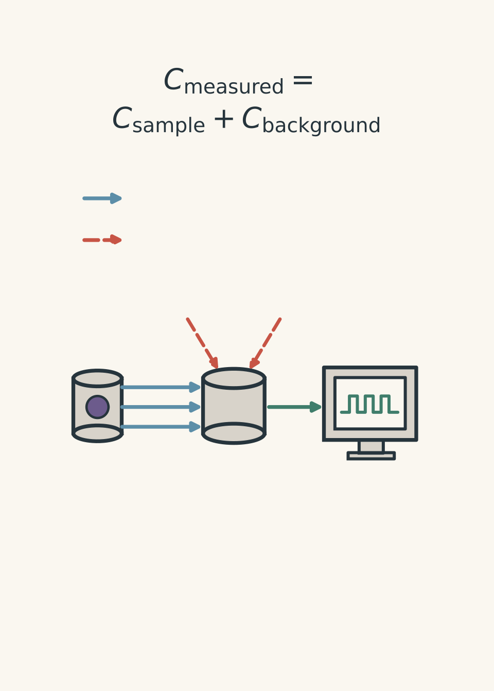
Worked example: Background plus a fractional half-life
A detector reads 700 counts/min from a radioactive sample. The background count rate is 100 counts/min. The sample’s half-life is 4.0 h. What should the detector read 10 h later, assuming the background and detector setup remain unchanged?
Step 1
\[ C_{\text{sample}} = 700-100 = 600\text{ counts/min} \]
The sample itself is initially contributing 600 counts/min.
Step 2
\[ n=\frac{10\text{ h}}{4.0\text{ h}} =2.5 \]
Step 3
\[ C_{\text{sample}} = 600\left(\frac12\right)^{2.5} \]
\[ C_{\text{sample}}\approx106\text{ counts/min} \]
Step 4
\[ C_{\text{measured}} = 106+100 \]
\[ C_{\text{measured}}\approx206\text{ counts/min} \]
The detector should therefore read about 206 counts/min.
A useful sanity check is that after 8 h, the sample would be at 150 counts/min. After another 2 h, it should be somewhere between 75 and 150 counts/min. About 106 fits that expectation. Then the constant 100 counts/min background brings the detector reading back up to about 206 counts/min.
05The traps that cause most half-life mistakes
1. Halving the wrong quantity
If the detector reads 900 counts/min and the background is 200 counts/min, you do not halve 900.
First find the sample contribution:
\[ 900-200=700\text{ counts/min} \]
Then apply radioactive decay to the 700.
2. Treating decay as linear
Radioactive decay does not remove the same number of nuclei every second.
It removes the same fraction over equal time intervals.
That is why a graph of amount against time curves downward rather than forming a straight line.
3. Forgetting to match the time units
A half-life of 30 min and a decay time of 2.0 h cannot be divided directly.
Convert first:
\[ 2.0\text{ h}=120\text{ min} \]
Then
\[ n=\frac{120}{30}=4 \]
4. Thinking half-life depends on the starting amount
A larger sample has more radioactive nuclei, so it has a larger initial activity. It does not have a longer half-life.
Half-life is a property of the radioactive isotope.
5. Assuming individual nuclei decay on schedule
A particular nucleus does not wait exactly one half-life and then decay. Half-life is a statistical description of a large collection of nuclei.
06When one half-life is not enough
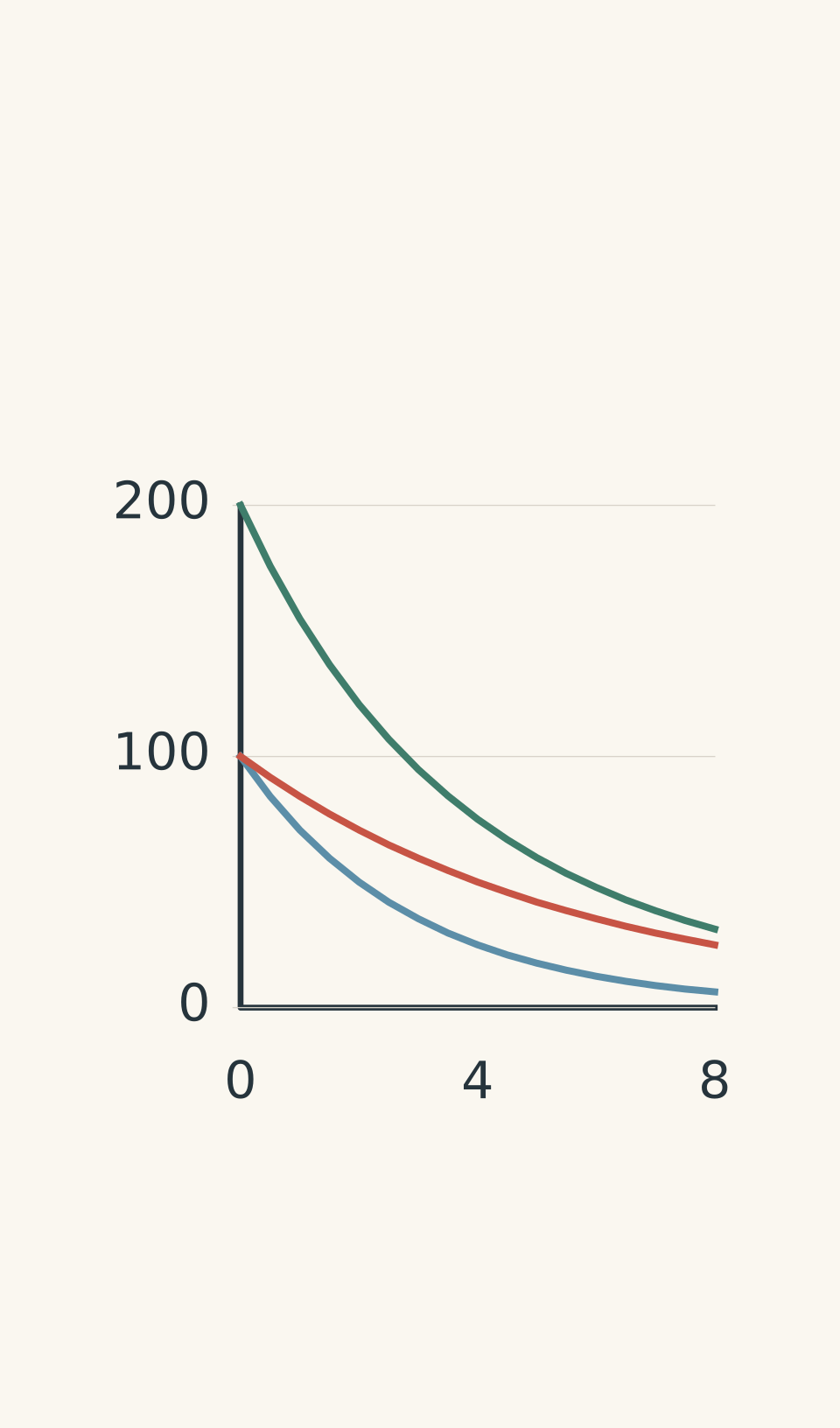
The repeated-halving model works cleanly when you are dealing with one radioactive isotope.
A mixture of different radioactive isotopes is different.
Suppose isotope A has a half-life of 2 h while isotope B has a half-life of 4 h. After 4 h:
- A has gone through two half-lives and has 25% of its original activity,
- B has gone through one half-life and has 50% of its original activity.
Their contributions are changing at different rates.
So the total activity of the mixture does not generally have one fixed half-life.
- Isotope A · half-life 2 h
- Isotope B · half-life 4 h
- Total mixture
This creates a useful exam warning: if a question gives you several isotopes, don’t automatically find one “overall half-life” by looking at the total reading.
For a deeper connection between half-life and the decay constant, see Decay constant and half-life: HSC Physics explained.
07Questions and solutions
Question 1
A radioactive isotope has a half-life of 3.0 h. A sample initially contains 960 mg of the radioactive isotope. What mass remains after 12 h?
Solution 1
60 mg remains. Four half-lives have passed, so the radioactive isotope has been reduced to \(1/16\) of its initial mass.
Step 1: Find the number of half-lives.
\[ n=\frac{12\text{ h}}{3.0\text{ h}}=4 \]
Step 2: Apply repeated halving.
\[ m=960\left(\frac12\right)^4 \]
\[ m=\frac{960}{16} =60\text{ mg} \]
The result means that 6.25% of the original radioactive isotope remains. The tempting mistake is to subtract 480 mg four times, but each half-life halves the current amount, not the original 960 mg.
Question 2
A detector records 720 counts/min when placed near a radioactive sample. The background count rate is 120 counts/min. The sample has a half-life of 5.0 h.
What should the detector record 15 h later, assuming the background and detector setup remain unchanged?
Solution 2
The detector should record 195 counts/min. The 120 counts/min background must be separated from the sample count rate before applying the half-life.
Step 1: Find the initial count rate due to the sample.
\[ C_{\text{sample},0} = 720-120 = 600\text{ counts/min} \]
Step 2: Find the number of half-lives.
\[ n=\frac{15\text{ h}}{5.0\text{ h}}=3 \]
Step 3: Apply three halvings to the sample contribution.
\[ C_{\text{sample}} = 600\left(\frac12\right)^3 \]
\[ C_{\text{sample}}=75\text{ counts/min} \]
Step 4: Add the unchanged background.
\[ C_{\text{measured}} = 75+120 = 195\text{ counts/min} \]
The trap is to apply the decay factor directly to 720 counts/min. That would incorrectly make the background decay along with the radioactive sample.
Question 3
Two radioactive samples are being compared.
- Sample A has a half-life of 3.0 h. Its activity is currently 500 Bq, after it has been decaying for 12 h.
- Sample B has a half-life of 6.0 h. Its activity is currently 600 Bq, after it has been decaying for 6.0 h.
Which sample had the greater initial activity? Which sample will have the greater activity 6.0 h from now?
Solution 3
Sample A started with the greater activity, at 8000 Bq. Six hours from now, however, sample B will have the greater activity, at 300 Bq compared with A’s 125 Bq. The current readings cannot be compared without accounting for each sample’s different decay history and half-life.
Step 1: Work backwards for sample A.
In 12 h, sample A has undergone
\[ n_A=\frac{12}{3.0}=4 \]
half-lives.
So 500 Bq is \(1/16\) of its initial activity:
\[ A_{A,0}=500\times16 =8000\text{ Bq} \]
Step 2: Work backwards for sample B.
In 6.0 h, sample B has undergone one half-life:
\[ A_{B,0}=600\times2 =1200\text{ Bq} \]
So sample A clearly began with more activity.
Step 3: Predict both samples 6.0 h from now.
For A, 6.0 h is two more half-lives:
\[ A_A=500\left(\frac12\right)^2 =125\text{ Bq} \]
For B, 6.0 h is one more half-life:
\[ A_B=600\left(\frac12\right) =300\text{ Bq} \]
Therefore B will be more active after another 6.0 h.
The important interaction is the different half-lives. A currently has 500 Bq, but it is decaying twice as fast in half-life terms, so its activity falls below B’s.
Question 4
At \(t=20\) h, a detector measures 900 counts/s from a radioactive sample. The background count rate is 100 counts/s. The sample has a half-life of 8.0 h.
What would the detector have read at \(t=0\)? What should it read at \(t=28\) h?
Assume the detector response and background remain constant.
Solution 4
The detector would have read about \(4.63\times10^3\) counts/s at \(t=0\), and it should read 500 counts/s at \(t=28\) h. The key is to remove the background first, then work backwards and forwards using the sample’s decay factor.
Step 1: Find the sample’s count rate at \(t=20\) h.
\[ C_{\text{sample}} = 900-100 = 800\text{ counts/s} \]
Step 2: Work backwards 20 h.
The number of half-lives is
\[ n=\frac{20}{8.0}=2.5 \]
So
\[ 800 = C_0\left(\frac12\right)^{2.5} \]
Rearranging,
\[ C_0 = 800\times2^{2.5} \]
\[ C_0\approx4525\text{ counts/s} \]
This is the sample’s count rate at \(t=0\).
Step 3: Restore the background.
\[ C_{\text{detector},0} = 4525+100 \]
\[ C_{\text{detector},0} \approx4625\text{ counts/s} \]
Step 4: Predict the reading at \(t=28\) h.
From 20 h to 28 h is exactly one half-life, so the sample count rate halves:
\[ C_{\text{sample},28} = \frac{800}{2} = 400\text{ counts/s} \]
Add the background:
\[ C_{\text{detector},28} = 400+100 = 500\text{ counts/s} \]
The tempting route is to halve the 900 counts/s detector reading. That would incorrectly make the background decay. Only the radioactive sample contribution follows the half-life.
Question 5
A sealed source contains two radioactive isotopes, A and B, and no other source of activity contributes to the measurements.
- Isotope A has a half-life of 2.0 h.
- Isotope B has a half-life of 4.0 h.
- At \(t=0\), the total activity is 10,000 Bq.
- At \(t=8.0\) h, the total activity is 1750 Bq.
Assume the measured activity is the sum of the two isotope activities and that the decay products do not contribute to the measured activity.
Determine the initial activity of A and the initial activity of B. Then predict the total activity at \(t=16\) h.
Finally, decide whether the source can be assigned one fixed half-life.
Solution 5
Isotope A initially had 4000 Bq, isotope B initially had 6000 Bq, and the total activity at 16 h will be about 391 Bq. The source cannot be described by one fixed half-life. The crucial point is that the two parts of the source are halving at different rates, so the total is the sum of two different decay patterns.
Step 1: Represent the initial activities.
Let \(R_A\) be the initial activity of isotope A and \(R_B\) the initial activity of isotope B.
At \(t=0\),
\[ R_A+R_B=10000 \]
Step 2: Work out how much of each isotope remains after 8.0 h.
For A:
\[ \frac{8.0}{2.0}=4 \]
half-lives have passed, so only \(1/16\) remains.
For B:
\[ \frac{8.0}{4.0}=2 \]
half-lives have passed, so \(1/4\) remains.
The measured total at 8.0 h is therefore
\[ \frac{R_A}{16} + \frac{R_B}{4} = 1750 \]
Step 3: Solve the two equations.
Multiply the second equation by 16:
\[ R_A+4R_B=28000 \]
We already know
\[ R_A+R_B=10000 \]
Subtracting gives
\[ 3R_B=18000 \]
so
\[ R_B=6000\text{ Bq} \]
Therefore
\[ R_A=10000-6000 \]
\[ R_A=4000\text{ Bq} \]
Step 4: Predict the total after another 8.0 h.
By 16 h, A has undergone eight half-lives:
\[ R_{A,16} = 4000\left(\frac12\right)^8 \]
\[ R_{A,16}=15.625\text{ Bq} \]
B has undergone four half-lives:
\[ R_{B,16} = 6000\left(\frac12\right)^4 \]
\[ R_{B,16}=375\text{ Bq} \]
Therefore
\[ R_{\text{total},16} = 15.625+375 \]
\[ R_{\text{total},16} = 390.625\text{ Bq} \]
So the total is about 391 Bq.
Step 5: Test the single-half-life idea.
A single half-life would mean that equal time intervals always multiply the total activity by the same factor.
From 0 to 8 h, the total changes by a factor of
\[ \frac{1750}{10000}=0.175 \]
If the whole source had one fixed half-life, the next 8 h should multiply the total by the same factor:
\[ 1750\times0.175 = 306.25\text{ Bq} \]
But the actual total is 390.625 Bq.
So one fixed half-life cannot describe the whole source.
The tempting route is to treat the 10,000 Bq and 1750 Bq readings as if they came from one radioactive isotope and fit a half-life to the total. The exact constraint that breaks this approach is that A and B have different half-lives. As time passes, the rapidly decaying A contribution becomes tiny, while the more persistent B contribution dominates. The total decay pattern therefore changes shape.
Once repeated halving is secure, the next useful step is to connect it to the decay constant \(\lambda\), which describes the same radioactive process continuously rather than only in half-life intervals.