
Black-body radiation and the ultraviolet catastrophe explained
Understand the shape of a black-body spectrum, why classical physics predicted an ultraviolet catastrophe, and how Planck's quantisation solved the problem.
Heat a piece of metal and its glow changes as the temperature rises: first dull red, then orange, then yellow-white. A simple classical prediction seems obvious. If hotter matter shakes charged particles more violently, perhaps shorter and shorter electromagnetic wavelengths should carry more and more energy. Push that reasoning far enough and the ultraviolet should dominate.
But it doesn’t. Real thermal spectra rise to a peak and then fall sharply at short wavelengths. Classical physics predicted the opposite – an unlimited increase in emitted energy. That failure became known as the ultraviolet catastrophe, and fixing it forced physicists to change what they thought energy could do.
01What does a black-body spectrum actually look like?
Imagine a hollow cavity with a tiny hole in one wall. Radiation entering the hole bounces around inside and is very unlikely to escape again. The hole therefore behaves almost like an ideal absorber.
If the cavity is held at a fixed temperature, radiation inside eventually reaches thermal equilibrium. The radiation coming out through the small hole has a spectrum determined mainly by the temperature, rather than by the material making the cavity.
That is the useful physical model behind a black body: an ideal object that absorbs all incident electromagnetic radiation and emits the characteristic thermal spectrum for its temperature.
Now make a prediction. If the temperature increases, what should happen to the spectrum?
Two things are observed:
- the object emits more energy overall, and
- the wavelength at which emission is strongest moves to a shorter wavelength.
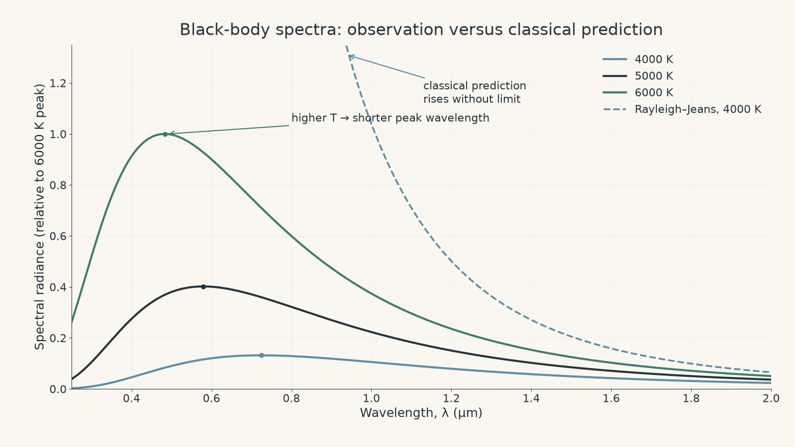
The spectrum is not a narrow spike. A hot object emits over a broad range of wavelengths. Its peak wavelength, \(\lambda_{\text{max}}\), is simply the wavelength where the curve reaches its maximum.
The shift of this peak is described by Wien’s displacement law:
\[ \lambda_{\text{max}}T=b \]
where:
- \(\lambda_{\text{max}}\) is the peak wavelength in metres,
- \(T\) is the absolute temperature in kelvin, and
- \(b=2.898\times10^{-3}\text{ m K}\) is Wien’s displacement constant.
So increasing \(T\) decreases \(\lambda_{\text{max}}\).
This explains the familiar change from red-hot to white-hot. It also tells us something more important: nature has a mechanism that prevents unlimited short-wavelength emission.
Worked example: Where does a hot filament emit most strongly?
A filament is at \(3000\text{ K}\). Calculate the wavelength at which its black-body spectrum peaks, and state whether this wavelength is visible.
Step 1
\[ \lambda_{\text{max}}T=b \]
Step 2
\[ \lambda_{\text{max}}=\frac{b}{T} \]
Step 3
\[ \lambda_{\text{max}} =\frac{2.898\times10^{-3}}{3000} =9.66\times10^{-7}\text{ m} \]
Step 4
\[ 9.66\times10^{-7}\text{ m}=966\text{ nm} \]
The peak is at about \(966\text{ nm}\), which is in the infrared.
That does not mean the filament emits no visible light. The spectrum is broad, so some radiation still falls in the visible range. The peak just happens to lie beyond red light.
02Why classical physics expected too much ultraviolet
To see where the classical prediction goes wrong, it helps to stop thinking about the surface of a glowing object and return to the cavity.
Electromagnetic waves can form standing-wave patterns inside the cavity. Only certain patterns fit, rather like the allowed standing waves on a guitar string, except that the cavity is three-dimensional and the waves are electromagnetic.
Each allowed standing-wave pattern is called a mode.
At low frequencies there are relatively few possible modes. At higher frequencies, many more different standing-wave patterns fit inside the cavity.
In fact, the number of modes available in a small frequency interval increases roughly as \(f^2\), where \(f\) is frequency.
So high frequency creates a dangerous combination:
- there are more modes available, and
- classical physics says each mode should receive roughly the same average thermal energy.
The second idea comes from the classical equipartition theorem.
For an electromagnetic mode in thermal equilibrium, classical statistical mechanics predicts an average energy
\[ \overline{E}=kT \]
where \(k=1.381\times10^{-23}\text{ J K}^{-1}\) is Boltzmann’s constant.
Picture an absurd school canteen rule: every student who turns up gets exactly one sandwich. That works while the number of students is finite. But now imagine that, as you walk towards the ultraviolet end of the queue, the number of students increases without limit. The sandwich budget becomes infinite.
Here, the students represent electromagnetic modes, and each sandwich represents the classical energy \(kT\).
The analogy breaks because energy is not literally handed out by someone, and electromagnetic modes are not independent hungry teenagers. The useful point is the counting: classical physics gives a non-zero average amount of energy to every available mode, while the number of high-frequency modes keeps increasing.
03The Rayleigh-Jeans prediction
Combining classical mode counting with equipartition gives the Rayleigh-Jeans law. Written in terms of frequency, the energy density per unit frequency is
\[ u(f,T)=\frac{8\pi f^2kT}{c^3} \]
where:
- \(u(f,T)\) describes how the radiation energy is distributed with frequency,
- \(f\) is frequency in hertz,
- \(T\) is temperature in kelvin,
- \(k\) is Boltzmann’s constant, and
- \(c\) is the speed of light.
Look at the important part:
\[ u(f,T)\propto f^2 \]
At a fixed temperature, doubling the frequency makes the classical prediction four times larger.
Triple the frequency and it becomes nine times larger.
As \(f\) approaches infinity, the predicted energy density also approaches infinity.
Because ultraviolet radiation has higher frequencies than visible light, this runaway high-frequency prediction became known as the ultraviolet catastrophe.
The “catastrophe” is a catastrophe for the theory, not for the actual object. A hot oven is not secretly firing an infinite amount of ultraviolet radiation into your kitchen.
04Why this prediction looked reasonable
The classical model was not foolish. It works well at sufficiently low frequencies.
That matters. A good replacement theory should not simply throw away successful classical physics. It should explain why the old theory worked in one region and failed in another.
Experimentally, the Rayleigh-Jeans prediction agrees reasonably well with black-body radiation at long wavelengths. The serious disagreement appears as the wavelength becomes shorter.
So the question becomes more precise:
Why should a high-frequency mode receive less thermal energy than classical equipartition predicts?
05Planck’s change: energy comes in frequency-dependent amounts
Max Planck introduced a new restriction. Energy exchange associated with a mode of frequency \(f\) occurs in discrete amounts related to
\[ E=hf \]
where \(h=6.626\times10^{-34}\text{ J s}\) is Planck’s constant.
More precisely, the allowed oscillator energies in Planck’s model could be written as
\[ E_n=nhf \]
where \(n=0,1,2,\ldots\).
The crucial feature is the size of one energy step:
\[ \Delta E=hf \]
A low-frequency mode has a small energy spacing. A high-frequency mode has a large energy spacing.
Think of an arcade where different games require different numbers of tokens before you can play. Classical equipartition effectively assumes every game can absorb arbitrary little amounts of energy. Planck’s rule says the high-frequency games have a much larger minimum token cost.
At a fixed temperature, thermal energy is limited. High-frequency modes are therefore much harder to excite.
The analogy breaks because a mode does not literally save up thermal “tokens”, but it captures the important competition: the quantum energy scale \(hf\) is being compared with the thermal energy scale \(kT\).
That comparison is one of the most useful ways to think about black-body radiation:
\[ \frac{hf}{kT} \]
If \(hf\ll kT\), the energy steps are small compared with the available thermal energy. Classical behaviour is a good approximation.
If \(hf\) becomes comparable with or larger than \(kT\), the discrete energy spacing matters strongly.
06How quantisation removes the catastrophe
Planck’s model gives the average energy of a cavity mode as
\[ \overline{E} = \frac{hf}{e^{hf/(kT)}-1} \]
This looks more complicated than the classical result \(kT\), but its physical message is clearer than the equation first appears.
At low frequency, \(hf\) is small compared with \(kT\). The expression approaches the classical value \(kT\).
At very high frequency, \(hf/(kT)\) becomes large. The exponential term in the denominator grows extremely quickly, so the average energy per high-frequency mode falls towards zero.
There are still many high-frequency modes.
The key change is that they are no longer each assigned \(kT\).
Combining Planck’s average mode energy with the same cavity mode counting gives
\[ u(f,T) = \frac{8\pi hf^3}{c^3} \frac{1}{e^{hf/(kT)}-1} \]
At first, increasing \(f\) creates more available modes, so the spectrum rises.
Eventually, however, the energy cost \(hf\) becomes too large compared with \(kT\). The exponential suppression wins, and the spectrum falls.
That produces a finite peak instead of an ultraviolet explosion.
Worked example: When does the classical approximation fail?
Consider thermal radiation at \(5800\text{ K}\), roughly the temperature scale of the Sun’s visible surface. Compare the quantum correction at a wavelength of \(10\,\mu\text{m}\) with that at \(200\text{ nm}\).
The ratio between Planck’s prediction and the corresponding classical Rayleigh-Jeans prediction at the same wavelength can be written as
\[ \frac{\text{Planck}}{\text{classical}} = \frac{x}{e^x-1} \]
where
\[ x=\frac{hc}{\lambda kT} \]
Step 1
Here,
\[ \lambda=10\,\mu\text{m}=1.0\times10^{-5}\text{ m} \]
so
\[ x= \frac{(6.626\times10^{-34})(3.00\times10^8)} {(1.0\times10^{-5})(1.381\times10^{-23})(5800)} \approx0.248 \]
Step 2
\[ \frac{x}{e^x-1} = \frac{0.248}{e^{0.248}-1} \approx0.88 \]
Planck’s result is about \(88\%\) of the classical prediction. The two models are reasonably close at this long wavelength.
Step 3
\[ \lambda=200\text{ nm}=2.00\times10^{-7}\text{ m} \]
\[ x= \frac{(6.626\times10^{-34})(3.00\times10^8)} {(2.00\times10^{-7})(1.381\times10^{-23})(5800)} \approx12.4 \]
Step 4
\[ \frac{x}{e^x-1} = \frac{12.4}{e^{12.4}-1} \approx5.1\times10^{-5} \]
At \(200\text{ nm}\), Planck’s prediction is only about \(0.005\%\) of the classical value.
That is the ultraviolet catastrophe in numerical form. The classical prediction does not become slightly inaccurate at short wavelengths. It eventually becomes wildly wrong.
07The most tempting misconception
A common interpretation is that Planck fixed the problem by adding a maximum allowed frequency.
He did not.
There is no hard wall where radiation suddenly becomes impossible. Black-body spectra have a smooth high-frequency tail.
The quantum model instead makes high-frequency excitations increasingly unlikely because the required energy step \(hf\) becomes large compared with \(kT\).
That difference matters. An arbitrary ultraviolet cut-off could prevent an infinite total energy, but it would not naturally reproduce the observed smooth spectrum and its systematic change with temperature.
08What increasing temperature really changes
Suppose the temperature increases.
It is tempting to say, “The spectrum moves to the left.”
That is incomplete.
A hotter black body emits more strongly across a broad range of wavelengths. At the same time, the peak moves towards shorter wavelengths.
The reason can again be seen from the competition between \(hf\) and \(kT\). Raising \(T\) increases the thermal energy scale \(kT\). Frequencies that were previously expensive compared with the available thermal energy become easier to excite.
So the high-frequency part of the spectrum becomes more populated, and the characteristic peak moves upwards in frequency, or downwards in wavelength.
Wien’s displacement law,
\[ \lambda_{\text{max}}T=b \]
is the measurable consequence.
09Classical and quantum predictions side by side
| Feature | Classical Rayleigh-Jeans model | Planck model | Observation |
|---|---|---|---|
| Long wavelengths | Works well | Approaches classical result | Matches both |
| High frequencies | Energy keeps increasing | High-frequency modes are strongly suppressed | Spectrum falls |
| Total emitted energy | Diverges if all frequencies are included | Finite | Finite |
| Spectrum has a peak | No finite high-frequency peak | Yes | Yes |
| Energy exchange | Effectively continuous | Quantised in steps related to \(hf\) | Quantum model matches spectrum |
| Effect of higher temperature | Greater classical energy per mode, but still ultraviolet divergence | Higher frequencies become easier to excite | Peak shifts to shorter wavelength |
The important lesson is not simply that “classical physics was wrong”. Classical physics is the low-frequency limit of the more complete quantum description.
10Questions and solutions
Question 1
A black body has a temperature of \(4000\text{ K}\).
Calculate its peak wavelength. A second black body is at \(8000\text{ K}\). Without repeating the full calculation, state the peak wavelength of the second object and explain the change.
Use \(b=2.898\times10^{-3}\text{ m K}\).
Solution 1
The \(4000\text{ K}\) body peaks at about \(725\text{ nm}\), while the \(8000\text{ K}\) body peaks at about \(362\text{ nm}\).
For the first object,
\[ \lambda_{\text{max}} = \frac{b}{T} = \frac{2.898\times10^{-3}}{4000} = 7.245\times10^{-7}\text{ m} \]
Therefore,
\[ \lambda_{\text{max}}\approx725\text{ nm} \]
For the second object, the temperature doubles. Since
\[ \lambda_{\text{max}}\propto\frac{1}{T} \]
doubling \(T\) halves the peak wavelength:
\[ \lambda_{\text{max}} = \frac{725}{2} \approx362\text{ nm} \]
The tempting mistake is to say that the hotter object’s entire spectrum has simply moved to \(362\text{ nm}\). It has not. The spectrum remains broad, its intensity increases, and its peak shifts to the shorter wavelength.
Question 2
According to the Rayleigh-Jeans law,
\[ u(f,T)=\frac{8\pi f^2kT}{c^3} \]
Two frequencies in the same cavity are \(3.0\times10^{14}\text{ Hz}\) and \(9.0\times10^{14}\text{ Hz}\).
At the same temperature:
- Calculate the ratio of the classical spectral energy densities at the two frequencies.
- Explain why extending this reasoning to arbitrarily high frequencies causes the ultraviolet catastrophe.
Solution 2
The Rayleigh-Jeans model predicts nine times as much spectral energy density at \(9.0\times10^{14}\text{ Hz}\) as at \(3.0\times10^{14}\text{ Hz}\), and its continued \(f^2\) growth produces an infinite total energy when all frequencies are included.
At constant temperature, all factors except \(f^2\) cancel:
\[ \frac{u_2}{u_1} = \frac{f_2^2}{f_1^2} \]
Substituting,
\[ \frac{u_2}{u_1} = \left( \frac{9.0\times10^{14}} {3.0\times10^{14}} \right)^2 = 3^2 = 9 \]
So
\[ u_2=9u_1 \]
The calculation itself is not yet a catastrophe. The problem appears when the same rule is applied without an upper limit.
As \(f\) increases,
\[ u(f,T)\propto f^2 \]
so the predicted energy density keeps increasing rather than turning over and falling.
The tempting route is to think, “Each individual frequency still has a finite value, so there is no problem.” The exact constraint that changes the conclusion is that a black-body spectrum contains a continuous range of frequencies. Adding the predicted contributions from higher and higher frequencies gives no finite total.
Real spectra instead fall sharply at high frequency.
Question 3
A cavity is at \(6000\text{ K}\). Compare radiation at \(500\text{ nm}\) and \(200\text{ nm}\) using
\[ x=\frac{hf}{kT}=\frac{hc}{\lambda kT} \]
Take \(h=6.626\times10^{-34}\text{ J s}\), \(c=3.00\times10^8\text{ m s}^{-1}\), and \(k=1.381\times10^{-23}\text{ J K}^{-1}\).
- Calculate \(x\) at each wavelength.
- State which wavelength is more strongly suppressed by quantum effects.
- Explain why classical equipartition becomes particularly poor in that case.
Solution 3
The values are approximately \(x=4.80\) at \(500\text{ nm}\) and \(x=12.0\) at \(200\text{ nm}\), so the \(200\text{ nm}\) radiation is much more strongly suppressed.
For \(500\text{ nm}\),
\[ \lambda=5.00\times10^{-7}\text{ m} \]
and
\[ x= \frac{(6.626\times10^{-34})(3.00\times10^8)} {(5.00\times10^{-7})(1.381\times10^{-23})(6000)} \approx4.80 \]
For \(200\text{ nm}\),
\[ \lambda=2.00\times10^{-7}\text{ m} \]
so
\[ x= \frac{(6.626\times10^{-34})(3.00\times10^8)} {(2.00\times10^{-7})(1.381\times10^{-23})(6000)} \approx12.0 \]
At \(200\text{ nm}\), the quantum energy scale \(hf\) is about twelve times the thermal scale \(kT\). Exciting such a mode therefore requires a relatively large energy step.
The tempting classical argument is that every mode should simply receive average energy \(kT\), regardless of frequency. That assumption ignores the fact that the minimum quantum energy spacing grows with frequency.
Because \(hf\gg kT\) at \(200\text{ nm}\), high-frequency excitation is unlikely. Planck’s expression therefore assigns those modes much less average energy than classical equipartition does.
Question 4
A student plots a black-body spectrum against wavelength and finds that the graph peaks at \(500\text{ nm}\).
They immediately claim that a graph of the same radiation against frequency must peak at
\[ f=\frac{c}{500\text{ nm}} \]
because wavelength and frequency satisfy \(c=f\lambda\).
Is that conclusion necessarily correct?
Use the fact that the energy contained in corresponding small intervals must satisfy
\[ B_\nu\,d\nu=B_\lambda\,|d\lambda| \]
and that
\[ \left|\frac{d\lambda}{d\nu}\right|=\frac{c}{\nu^2} \]
where \(B_\lambda\) is spectral radiance per unit wavelength and \(B_\nu\) is spectral radiance per unit frequency.
Solution 4
No. The frequency spectrum does not generally peak at the simple reciprocal of the wavelength-spectrum peak.
The relation
\[ c=f\lambda \]
correctly maps an individual wavelength to an individual frequency. The trap is assuming that the vertical axis remains unchanged when the horizontal variable is changed.
The spectrum describes energy per interval. Equal wavelength intervals do not correspond to equal frequency intervals.
From
\[ B_\nu\,d\nu=B_\lambda\,|d\lambda| \]
we obtain
\[ B_\nu = B_\lambda \left|\frac{d\lambda}{d\nu}\right| \]
and therefore
\[ B_\nu = B_\lambda\frac{c}{\nu^2} \]
Equivalently, because \(\lambda=c/\nu\),
\[ B_\nu=B_\lambda\frac{\lambda^2}{c} \]
The multiplying factor is not constant across the spectrum. It changes with wavelength or frequency.
That changes the shape of the graph and therefore changes the position of its maximum.
The tempting route is to treat a spectrum as if it were a collection of points that can simply be relabelled along the horizontal axis. The exact issue is that each plotted height means “energy per unit of horizontal-axis interval”. Changing from wavelength intervals to frequency intervals changes those interval sizes.
This does not change the physical radiation. It changes how the same radiation is represented.
Question 5
Suppose you do not know Planck’s exact formula. You only know that a successful theory must reduce the average energy per cavity mode below the classical value at sufficiently high frequency.
A theorist proposes the general form
\[ \overline{E} = kT\, g\left(\frac{hf}{kT}\right) \]
where \(g(x)\) has these properties:
- \(g(x)\rightarrow1\) when \(x\ll1\),
- \(g(x)\) falls rapidly towards zero when \(x\gg1\).
The number of electromagnetic modes per unit frequency still increases in proportion to \(f^2\).
Without knowing the exact mathematical form of \(g\):
- Explain why this model recovers the Rayleigh-Jeans result at low frequency.
- Explain how it can avoid the ultraviolet catastrophe.
- Show why the characteristic frequency of the spectrum must be proportional to \(T\).
- Hence explain why a characteristic wavelength must be proportional to \(1/T\).
- Predict how the total radiation energy density scales with temperature, using the shape of the spectrum rather than a detailed integration.
Solution 5
The model automatically gives classical behaviour at low frequency, suppresses sufficiently high frequencies, predicts \(f_{\text{characteristic}}\propto T\), predicts \(\lambda_{\text{characteristic}}\propto1/T\), and gives total radiation energy proportional to \(T^4\).
Start with the proposed average mode energy:
\[ \overline{E} = kT\, g\left(\frac{hf}{kT}\right) \]
At low frequency,
\[ \frac{hf}{kT}\ll1 \]
so the given rule says
\[ g\left(\frac{hf}{kT}\right)\rightarrow1 \]
Therefore,
\[ \overline{E}\rightarrow kT \]
which is exactly the classical equipartition result. Since the density of modes is still proportional to \(f^2\),
\[ u(f,T)\propto f^2kT \]
and the Rayleigh-Jeans behaviour is recovered.
At high frequency,
\[ \frac{hf}{kT}\gg1 \]
and \(g\) falls rapidly towards zero. Although the number of modes continues to grow as \(f^2\), their average energy can fall quickly enough for the high-frequency tail to decrease rather than diverge.
That is the crucial competition. Merely having more modes does not force an ultraviolet catastrophe if the energy per mode falls sufficiently fast.
Now define
\[ x=\frac{hf}{kT} \]
A particular feature of the spectrum – for example its peak – will occur at some particular value of \(x\), say \(x=x_0\), provided the function \(g\) itself does not change with temperature.
Then
\[ x_0=\frac{hf_{\text{peak}}}{kT} \]
so
\[ f_{\text{peak}} = \frac{x_0k}{h}T \]
Everything multiplying \(T\) is constant. Therefore,
\[ f_{\text{peak}}\propto T \]
Since wavelength and frequency are related by
\[ \lambda=\frac{c}{f} \]
it follows that
\[ \lambda_{\text{peak}}\propto\frac{1}{T} \]
This is the structure behind Wien’s displacement law.
There is one more result hidden in the same reasoning. The spectrum has the form
\[ u(f,T)\propto f^2kT\, g\left(\frac{hf}{kT}\right) \]
For a fixed value of the scaled variable \(x\), frequency is proportional to \(T\). Therefore the \(f^2kT\) part gives a vertical scale proportional to
\[ T^2\times T=T^3 \]
Meanwhile, because characteristic frequencies are proportional to \(T\), the horizontal width of the spectrum on a frequency graph also scales as \(T\).
So the area under the spectrum scales as
\[ T^3\times T=T^4 \]
Hence the total radiation energy density is proportional to
\[ T^4 \]
The tempting answer is that Planck’s solution merely “cuts off the ultraviolet”. This general argument shows something deeper. A successful quantum correction connects frequency and temperature through the ratio \(hf/(kT)\). That single comparison explains why classical physics reappears at low frequency, why the ultraviolet divergence disappears, why the spectral peak shifts with temperature, and why the total emitted energy grows so rapidly as an object becomes hotter.
That same idea – comparing a quantum energy scale such as \(hf\) with another physically available energy scale – becomes useful again when studying photons and the photoelectric effect.