
Predicting Precipitation with Ksp for HSC Chemistry
Learn how to use ion concentrations, Qsp, and Ksp to predict whether a precipitate forms after solutions are mixed. Includes worked examples and challenging HSC-style questions.
Two clear solutions can be perfectly stable on their own, then turn cloudy the moment you mix them. The obvious explanation is that an insoluble salt has formed. The harder HSC question is more precise: was there actually enough of each ion present for precipitation to occur?
Suppose a mixed solution contains \([\mathrm{Ag}^{+}] = 1.0 \times 10^{-5}\) mol L\(^{-1}\) and \([\mathrm{Cl}^{-}] = 1.0 \times 10^{-5}\) mol L\(^{-1}\). Would you expect \(\ce{AgCl}\) to precipitate?
You might say yes because silver chloride is usually described as insoluble. But those concentrations give an ion product of only \(1.0 \times 10^{-10}\), below the \(K_{sp}\) of \(\ce{AgCl}\), about \(1.8 \times 10^{-10}\) at 25 °C. The solution can hold those ions without forming a precipitate.
That is the point of \(K_{sp}\): it turns a qualitative idea like “sparingly soluble” into a quantitative decision.
01Think about ion crowding first
Imagine the dissolved ions are people at a slightly awkward school formal. There isn’t a separate maximum number of \(\mathrm{Ag}^{+}\) ions and a separate maximum number of \(\mathrm{Cl}^{-}\) ions. What matters is the combination.
If there are very few chloride ions around, a larger concentration of silver ions can remain dissolved. If both are present at substantial concentrations, the combination can become too large to remain at equilibrium, and solid \(\ce{AgCl}\) forms.
The analogy breaks because ions are not literally pairing off like Year 12 students trying to avoid eye contact. More importantly, not every solid has a 1:1 formula. For \(\ce{CaF2}\), two fluoride ions are involved for every calcium ion, so the fluoride concentration gets squared in the equilibrium expression.
That stoichiometry is where \(K_{sp}\) becomes more useful than a simple solubility rule.
If you need the qualitative starting point first, see Solubility Rules and Precipitation Tests for HSC Chemistry.
02From dissolution equilibrium to \(K_{sp}\)
Consider silver chloride:
\[ \ce{AgCl(s) <=> Ag+(aq) + Cl-(aq)} \]
At equilibrium,
\[ K_{sp} = [\mathrm{Ag}^{+}][\mathrm{Cl}^{-}] \]
Here:
- \(K_{sp}\) is the solubility product constant,
- \([\mathrm{Ag}^{+}]\) is the equilibrium concentration of silver ions in mol L\(^{-1}\),
- \([\mathrm{Cl}^{-}]\) is the equilibrium concentration of chloride ions in mol L\(^{-1}\).
The solid does not appear in the \(K_{sp}\) expression.
Now compare that with calcium fluoride:
\[ \ce{CaF2(s) <=> Ca^2+(aq) + 2F-(aq)} \]
so
\[ K_{sp} = [\mathrm{Ca}^{2+}][\mathrm{F}^{-}]^2 \]
The power of 2 comes directly from the coefficient of \(\mathrm{F}^{-}\) in the dissolution equation.
This is not optional bookkeeping. Forgetting the square can completely reverse your prediction.
Some commonly tabulated values at 25 °C are:
| Solid | Dissolution equilibrium | \(K_{sp}\) |
|---|---|---|
| \(\ce{AgCl}\) | \(\ce{AgCl(s) <=> Ag+(aq) + Cl-(aq)}\) | \(1.8 \times 10^{-10}\) |
| \(\ce{BaSO4}\) | \(\ce{BaSO4(s) <=> Ba^2+(aq) + SO4^2-(aq)}\) | \(1.1 \times 10^{-10}\) |
| \(\ce{CaF2}\) | \(\ce{CaF2(s) <=> Ca^2+(aq) + 2F-(aq)}\) | \(3.9 \times 10^{-11}\) |
| \(\ce{Ag2CrO4}\) | \(\ce{Ag2CrO4(s) <=> 2Ag+(aq) + CrO4^2-(aq)}\) | \(1.1 \times 10^{-12}\) |
Different data sources can give slightly different values because \(K_{sp}\) depends on temperature and experimental conditions. In an HSC question, use the value supplied in the question or data provided.
03\(Q_{sp}\) asks a different question
\(K_{sp}\) describes the equilibrium boundary.
To decide whether a mixture is currently above or below that boundary, calculate the ion product, \(Q_{sp}\).
For \(\ce{AgCl}\),
\[ Q_{sp} = [\mathrm{Ag}^{+}][\mathrm{Cl}^{-}] \]
It has exactly the same form as the \(K_{sp}\) expression. The difference is what concentrations you put into it.
For \(K_{sp}\), the concentrations are equilibrium concentrations in a saturated system.
For \(Q_{sp}\), use the ion concentrations that exist now, usually immediately after mixing and before any precipitation has occurred.
Then compare:
| Comparison | Meaning | Prediction |
|---|---|---|
| \(Q_{sp} < K_{sp}\) | The solution is unsaturated | No precipitate forms |
| \(Q_{sp} = K_{sp}\) | The solution is at the saturation boundary | No net precipitation is required |
| \(Q_{sp} > K_{sp}\) | The solution is supersaturated with respect to that solid | Precipitation is favoured |
If \(Q_{sp} > K_{sp}\), ions leave the solution as solid until the dissolved ion concentrations have fallen enough for equilibrium to be restored.
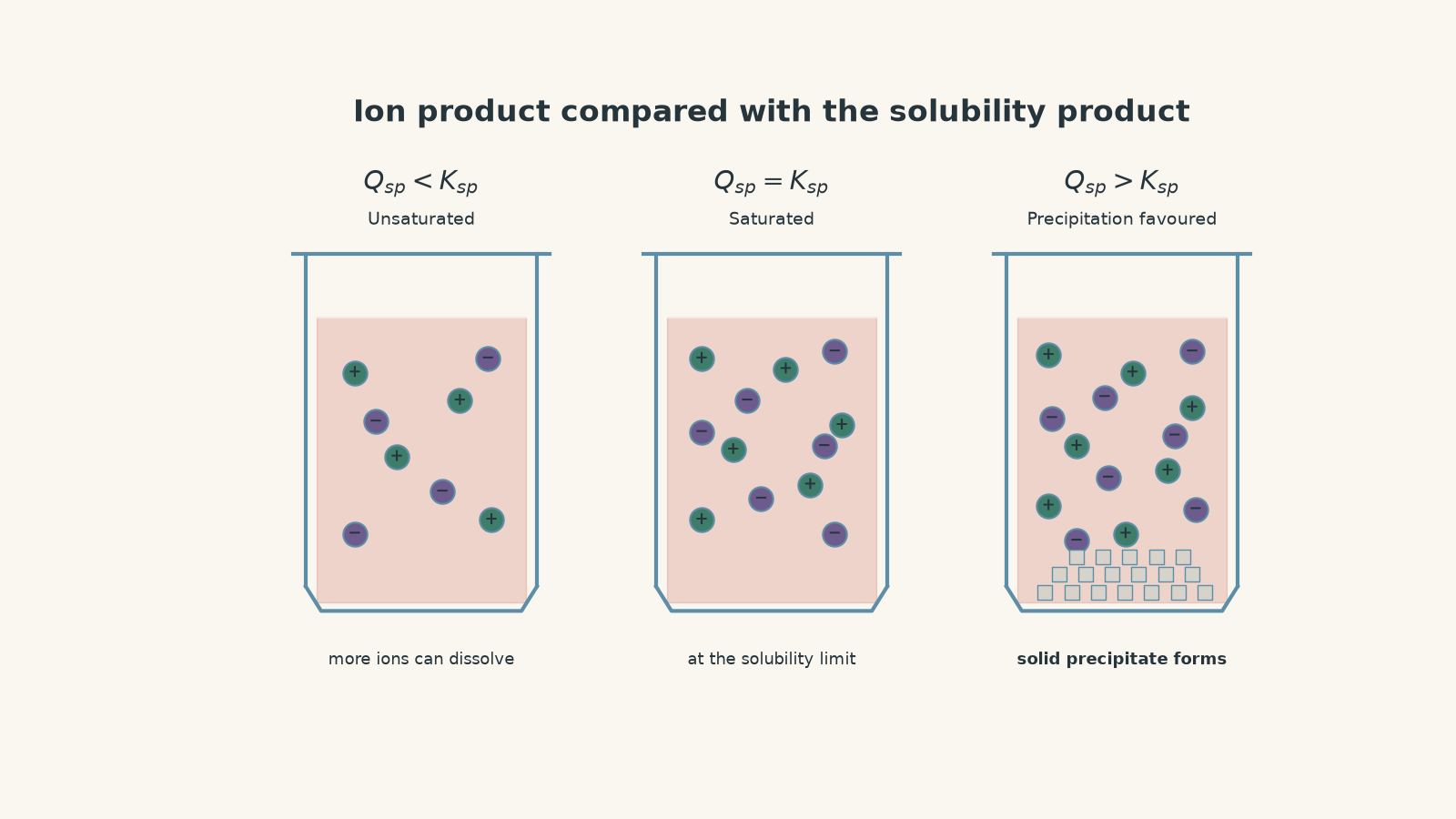
There is one layer of precision worth adding. Real precipitation can require nucleation, so a supersaturated solution can sometimes persist temporarily. HSC equilibrium questions normally ignore that kinetic delay and predict precipitation when \(Q_{sp}>K_{sp}\).
04The calculation most students skip: dilution after mixing
Suppose you mix 20 mL of one solution with 30 mL of another.
The ions from the first solution are no longer confined to 20 mL. They are now spread through approximately 50 mL.
So you usually cannot take the two concentrations printed in the question and place them straight into \(Q_{sp}\).
Refresh the concentration relationship:
\[ n = cV \]
where:
- \(n\) is amount in mol,
- \(c\) is concentration in mol L\(^{-1}\),
- \(V\) is volume in L.
After mixing,
\[ c_{\text{after mixing}} = \frac{n}{V_{\text{total}}} \]
For ordinary HSC aqueous-solution questions, volumes are usually assumed to be additive unless told otherwise.
A reliable precipitation method is therefore:
- Write the possible precipitation equilibrium.
- Write the \(Q_{sp}\) expression from the coefficients.
- Find the moles of each relevant ion before mixing.
- Divide those moles by the total mixed volume.
- Calculate \(Q_{sp}\).
- Compare \(Q_{sp}\) with \(K_{sp}\).
Spectator ions do not appear in the \(Q_{sp}\) expression.
Worked example: Will silver chloride precipitate after mixing?
20.0 mL of \(2.00 \times 10^{-4}\) mol L\(^{-1}\) \(\ce{AgNO3}\) is mixed with 30.0 mL of \(1.00 \times 10^{-4}\) mol L\(^{-1}\) \(\ce{NaCl}\). Predict whether \(\ce{AgCl}\) precipitates at 25 °C. Use \(K_{sp}(\ce{AgCl}) = 1.8 \times 10^{-10}\).
Step 1
\[ \ce{AgCl(s) <=> Ag+(aq) + Cl-(aq)} \]
Therefore,
\[ Q_{sp} = [\mathrm{Ag}^{+}][\mathrm{Cl}^{-}] \]
Step 2
For silver ions:
\[ n(\mathrm{Ag}^{+}) = cV = (2.00 \times 10^{-4})(0.0200) = 4.00 \times 10^{-6}\ \mathrm{mol} \]
For chloride ions:
\[ n(\mathrm{Cl}^{-}) = (1.00 \times 10^{-4})(0.0300) = 3.00 \times 10^{-6}\ \mathrm{mol} \]
Step 3
\[ V_{\text{total}} = 0.0200 + 0.0300 = 0.0500\ \mathrm{L} \]
Therefore,
\[ [\mathrm{Ag}^{+}] = \frac{4.00 \times 10^{-6}}{0.0500} = 8.00 \times 10^{-5}\ \mathrm{mol\,L^{-1}} \]
and
\[ [\mathrm{Cl}^{-}] = \frac{3.00 \times 10^{-6}}{0.0500} = 6.00 \times 10^{-5}\ \mathrm{mol\,L^{-1}} \]
Step 4
\[ Q_{sp} = (8.00 \times 10^{-5})(6.00 \times 10^{-5}) = 4.80 \times 10^{-9} \]
Step 5
\[ 4.80 \times 10^{-9} > 1.8 \times 10^{-10} \]
Therefore, \(\ce{AgCl}\) precipitates.
The useful interpretation is not simply “silver chloride is insoluble”. The mixed solution initially contains more dissolved \(\mathrm{Ag}^{+}\) and \(\mathrm{Cl}^{-}\) together than equilibrium permits.
Worked example: Does calcium fluoride precipitate?
30.0 mL of \(1.00 \times 10^{-3}\) mol L\(^{-1}\) \(\ce{CaCl2}\) is mixed with 20.0 mL of \(2.00 \times 10^{-3}\) mol L\(^{-1}\) \(\ce{NaF}\). Predict whether \(\ce{CaF2}\) precipitates. Use \(K_{sp}(\ce{CaF2}) = 3.9 \times 10^{-11}\).
Step 1
\[ \ce{CaF2(s) <=> Ca^2+(aq) + 2F-(aq)} \]
So,
\[ Q_{sp} = [\mathrm{Ca}^{2+}][\mathrm{F}^{-}]^2 \]
That square is the main extra difficulty.
Step 2
\[ n(\mathrm{Ca}^{2+}) = (1.00 \times 10^{-3})(0.0300) = 3.00 \times 10^{-5}\ \mathrm{mol} \]
\[ n(\mathrm{F}^{-}) = (2.00 \times 10^{-3})(0.0200) = 4.00 \times 10^{-5}\ \mathrm{mol} \]
The fact that \(\ce{CaCl2}\) contains two chloride ions does not double the calcium concentration. One mole of \(\ce{CaCl2}\) provides one mole of \(\mathrm{Ca}^{2+}\).
Similarly, one mole of \(\ce{NaF}\) provides one mole of \(\mathrm{F}^{-}\).
Step 3
The total volume is
\[ V_{\text{total}} = 0.0300 + 0.0200 = 0.0500\ \mathrm{L} \]
Therefore,
\[ [\mathrm{Ca}^{2+}] = \frac{3.00 \times 10^{-5}}{0.0500} = 6.00 \times 10^{-4}\ \mathrm{mol\,L^{-1}} \]
and
\[ [\mathrm{F}^{-}] = \frac{4.00 \times 10^{-5}}{0.0500} = 8.00 \times 10^{-4}\ \mathrm{mol\,L^{-1}} \]
Step 4
\[ Q_{sp} = (6.00 \times 10^{-4})(8.00 \times 10^{-4})^2 = 3.84 \times 10^{-10} \]
Step 5
\[ 3.84 \times 10^{-10} > 3.9 \times 10^{-11} \]
Therefore, \(\ce{CaF2}\) precipitates.
Notice that \(Q_{sp}\) is almost ten times \(K_{sp}\). The solution must reduce the combination \([\mathrm{Ca}^{2+}][\mathrm{F}^{-}]^2\), which it does by removing calcium and fluoride ions into solid \(\ce{CaF2}\).
05Why the obvious shortcuts fail
The most tempting mistake is to look at a concentration and compare it directly with \(K_{sp}\).
For example, saying
\[ [\mathrm{Ag}^{+}] = 8.0 \times 10^{-5} > 1.8 \times 10^{-10} \]
tells you nothing useful. \(K_{sp}\) is not a maximum concentration of one particular ion. It constrains a combination of ion concentrations.
A second common mistake is to use the original concentrations before mixing. That usually makes \(Q_{sp}\) too large because it ignores dilution.
A third is to forget stoichiometric powers. For calcium fluoride,
\[ Q_{sp} = [\mathrm{Ca}^{2+}][\mathrm{F}^{-}]^2 \]
not
\[ Q_{sp} = [\mathrm{Ca}^{2+}][\mathrm{F}^{-}] \]
A fourth mistake is subtler: assuming that \(Q_{sp}>K_{sp}\) means every possible dissolved ion precipitates. It does not. Precipitation continues only until equilibrium is reached. Some of each ion generally remains dissolved.
This becomes important when one reactant seems to be the “limiting ion”. Stoichiometry may consume almost all of it, but equilibrium prevents its concentration from becoming literally zero.
06A quick decision rule
When a precipitation question gives you two solutions to mix, your scratch working should usually have this shape:
\[ \text{moles before mixing} \rightarrow \text{concentrations after mixing} \rightarrow Q_{sp} \rightarrow \text{compare with }K_{sp} \]
Do not reverse the middle two steps.
If the question instead gives concentrations that already refer to the final mixture, you can calculate \(Q_{sp}\) directly. Reading exactly what each concentration describes can save half a page of unnecessary working.
07Questions and solutions
Question 1
25.0 mL of \(4.0 \times 10^{-4}\) mol L\(^{-1}\) \(\ce{BaCl2}\) is mixed with 25.0 mL of \(2.0 \times 10^{-4}\) mol L\(^{-1}\) \(\ce{Na2SO4}\).
Using \(K_{sp}(\ce{BaSO4}) = 1.1 \times 10^{-10}\), determine whether a precipitate forms.
Solution 1
A \(\ce{BaSO4}\) precipitate forms because the ion product after mixing is greater than \(K_{sp}\).
The equilibrium is
\[ \ce{BaSO4(s) <=> Ba^2+(aq) + SO4^2-(aq)} \]
so
\[ Q_{sp} = [\mathrm{Ba}^{2+}][\mathrm{SO_{4}}^{2-}] \]
Because equal volumes are mixed, each original ion concentration is halved.
\[ [\mathrm{Ba}^{2+}] = 2.0 \times 10^{-4}\ \mathrm{mol\,L^{-1}} \]
\[ [\mathrm{SO_{4}}^{2-}] = 1.0 \times 10^{-4}\ \mathrm{mol\,L^{-1}} \]
Therefore,
\[ Q_{sp} = (2.0 \times 10^{-4})(1.0 \times 10^{-4}) = 2.0 \times 10^{-8} \]
Comparing:
\[ 2.0 \times 10^{-8} > 1.1 \times 10^{-10} \]
so \(\ce{BaSO4(s)}\) forms.
The tempting shortcut is to multiply the two original concentrations without allowing for dilution. That would still predict precipitation here, but it would give the wrong \(Q_{sp}\), and the same mistake can reverse an answer when the values are closer to the threshold.
Question 2
10.0 mL of \(1.00 \times 10^{-3}\) mol L\(^{-1}\) \(\ce{CaCl2}\) is mixed with 40.0 mL of a \(\ce{NaF}\) solution.
Use \(K_{sp}(\ce{CaF2}) = 3.9 \times 10^{-11}\).
What is the greatest initial concentration of the \(\ce{NaF}\) solution that can be mixed with the \(\ce{CaCl2}\) without causing \(\ce{CaF2}\) to precipitate?
Assume volumes are additive.
Solution 2
The greatest allowable initial \(\ce{NaF}\) concentration is approximately \(5.52 \times 10^{-4}\) mol L\(^{-1}\). At this concentration, the final mixture is exactly at the precipitation threshold.
For calcium fluoride,
\[ K_{sp} = [\mathrm{Ca}^{2+}][\mathrm{F}^{-}]^2 \]
First find the calcium concentration after mixing.
The initial amount of \(\mathrm{Ca}^{2+}\) is
\[ n = (1.00 \times 10^{-3})(0.0100) = 1.00 \times 10^{-5}\ \mathrm{mol} \]
The total volume is
\[ 0.0100 + 0.0400 = 0.0500\ \mathrm{L} \]
so
\[ [\mathrm{Ca}^{2+}] = \frac{1.00 \times 10^{-5}}{0.0500} = 2.00 \times 10^{-4}\ \mathrm{mol\,L^{-1}} \]
Let the initial concentration of the \(\ce{NaF}\) solution be \(C\) mol L\(^{-1}\).
After 40.0 mL is diluted to 50.0 mL,
\[ [\mathrm{F}^{-}] = C\left(\frac{40.0}{50.0}\right) = 0.800C \]
At the exact point where precipitation is about to begin,
\[ Q_{sp}=K_{sp} \]
Therefore,
\[ (2.00 \times 10^{-4})(0.800C)^2 = 3.9 \times 10^{-11} \]
\[ 1.28 \times 10^{-4}C^2 = 3.9 \times 10^{-11} \]
\[ C^2 = 3.046875 \times 10^{-7} \]
\[ C = 5.52 \times 10^{-4}\ \mathrm{mol\,L^{-1}} \]
Thus an initial concentration at or below approximately \(5.52 \times 10^{-4}\) mol L\(^{-1}\) does not require precipitation in the HSC equilibrium model. Any larger concentration gives \(Q_{sp}>K_{sp}\).
A tempting route is to set the original fluoride concentration directly equal to the equilibrium fluoride concentration. The constraint that changes the result is dilution: the fluoride solution occupies 40.0 mL before mixing but 50.0 mL afterwards.
Question 3
50.0 mL of \(1.00 \times 10^{-3}\) mol L\(^{-1}\) \(\ce{AgNO3}\) is mixed with 50.0 mL of \(6.00 \times 10^{-4}\) mol L\(^{-1}\) \(\ce{NaCl}\).
Use \(K_{sp}(\ce{AgCl}) = 1.8 \times 10^{-10}\).
Determine:
a. whether \(\ce{AgCl}\) precipitates,
b. which ion is in stoichiometric excess, and
c. the approximate equilibrium concentrations of \(\mathrm{Ag}^{+}\) and \(\mathrm{Cl}^{-}\) after precipitation.
Assume the total volume remains 100.0 mL.
Solution 3
\(\ce{AgCl}\) precipitates, \(\mathrm{Ag}^{+}\) is in stoichiometric excess, and the final concentrations are approximately \([\mathrm{Ag}^{+}] = 2.01 \times 10^{-4}\) mol L\(^{-1}\) and \([\mathrm{Cl}^{-}] = 8.96 \times 10^{-7}\) mol L\(^{-1}\).
First check that precipitation occurs.
After equal-volume mixing,
\[ [\mathrm{Ag}^{+}]_{\text{initial mixture}} = 5.00 \times 10^{-4}\ \mathrm{mol\,L^{-1}} \]
and
\[ [\mathrm{Cl}^{-}]_{\text{initial mixture}} = 3.00 \times 10^{-4}\ \mathrm{mol\,L^{-1}} \]
Therefore,
\[ Q_{sp} = (5.00 \times 10^{-4})(3.00 \times 10^{-4}) = 1.50 \times 10^{-7} \]
Since
\[ 1.50 \times 10^{-7} > 1.8 \times 10^{-10}, \]
precipitation occurs.
Now compare initial amounts:
\[ n(\mathrm{Ag}^{+}) = (1.00 \times 10^{-3})(0.0500) = 5.00 \times 10^{-5}\ \mathrm{mol} \]
\[ n(\mathrm{Cl}^{-}) = (6.00 \times 10^{-4})(0.0500) = 3.00 \times 10^{-5}\ \mathrm{mol} \]
The precipitation equation is
\[ \ce{Ag+(aq) + Cl-(aq) -> AgCl(s)} \]
so the ions react in a 1:1 ratio.
After the main stoichiometric precipitation step, approximately
\[ 5.00 \times 10^{-5} - 3.00 \times 10^{-5} = 2.00 \times 10^{-5}\ \mathrm{mol} \]
of \(\mathrm{Ag}^{+}\) remains.
In 0.1000 L,
\[ [\mathrm{Ag}^{+}] \approx 2.00 \times 10^{-4}\ \mathrm{mol\,L^{-1}} \]
It is tempting now to say \([\mathrm{Cl}^{-}]=0\). That would violate the equilibrium condition. If solid \(\ce{AgCl}\) is present,
\[ [\mathrm{Ag}^{+}][\mathrm{Cl}^{-}] = 1.8 \times 10^{-10} \]
Using the approximate silver concentration,
\[ [\mathrm{Cl}^{-}] \approx \frac{1.8 \times 10^{-10}}{2.00 \times 10^{-4}} = 9.0 \times 10^{-7}\ \mathrm{mol\,L^{-1}} \]
A slightly more precise treatment allows the small amount of dissolved \(\ce{AgCl}\) to increase both ion concentrations.
Let the equilibrium chloride concentration be \(x\). Then
\[ [\mathrm{Ag}^{+}] = 2.00 \times 10^{-4}+x \]
and
\[ x(2.00 \times 10^{-4}+x) = 1.8 \times 10^{-10} \]
Solving gives
\[ x = 8.96 \times 10^{-7}\ \mathrm{mol\,L^{-1}} \]
so
\[ [\mathrm{Cl}^{-}] = 8.96 \times 10^{-7}\ \mathrm{mol\,L^{-1}} \]
and
\[ [\mathrm{Ag}^{+}] = 2.009 \times 10^{-4}\ \mathrm{mol\,L^{-1}} \approx 2.01 \times 10^{-4}\ \mathrm{mol\,L^{-1}} \]
The trap is treating stoichiometric completion as equilibrium completion. Stoichiometry tells you which ion is nearly removed. \(K_{sp}\) tells you that its dissolved concentration cannot simply be set to zero while the solid and the other ion remain present.
Question 4
At 25 °C, a saturated solution of \(\ce{CaF2}\) is filtered so that no solid \(\ce{CaF2}\) remains in the filtrate.
Use \(K_{sp}(\ce{CaF2}) = 3.9 \times 10^{-11}\).
a. Calculate \([\mathrm{Ca}^{2+}]\) and \([\mathrm{F}^{-}]\) in the saturated filtrate.
b. A 50.0 mL sample of this filtrate is mixed with 50.0 mL of \(0.0100\) mol L\(^{-1}\) \(\ce{CaCl2}\). Predict whether \(\ce{CaF2}\) precipitates.
c. A separate 50.0 mL sample of the same saturated filtrate is instead mixed with 50.0 mL of pure water. Predict whether a precipitate forms.
d. If undissolved \(\ce{CaF2}\) had not been filtered out before the dilution in part c, what would happen to some of that existing solid?
Solution 4
Adding the \(\ce{CaCl2}\) causes \(\ce{CaF2}\) to precipitate, while adding pure water makes the solution unsaturated. If undissolved \(\ce{CaF2}\) were present during the water dilution, some of that solid would dissolve.
For the original saturated solution,
\[ \ce{CaF2(s) <=> Ca^2+(aq) + 2F-(aq)} \]
Let the molar solubility be \(s\) mol L\(^{-1}\).
Then
\[ [\mathrm{Ca}^{2+}] = s \]
and
\[ [\mathrm{F}^{-}] = 2s \]
Therefore,
\[ K_{sp} = s(2s)^2 = 4s^3 \]
so
\[ 4s^3 = 3.9 \times 10^{-11} \]
\[ s = \left(\frac{3.9 \times 10^{-11}}{4}\right)^{1/3} = 2.14 \times 10^{-4}\ \mathrm{mol\,L^{-1}} \]
Thus,
\[ [\mathrm{Ca}^{2+}] = 2.14 \times 10^{-4}\ \mathrm{mol\,L^{-1}} \]
and
\[ [\mathrm{F}^{-}] = 4.27 \times 10^{-4}\ \mathrm{mol\,L^{-1}} \]
For part b, mixing equal volumes halves the fluoride concentration, but the second solution also supplies a large amount of calcium.
Immediately after mixing,
\[ [\mathrm{F}^{-}] = \frac{4.27 \times 10^{-4}}{2} = 2.14 \times 10^{-4}\ \mathrm{mol\,L^{-1}} \]
The calcium comes from both solutions:
\[ [\mathrm{Ca}^{2+}] = \frac{2.14 \times 10^{-4}+0.0100}{2} = 5.11 \times 10^{-3}\ \mathrm{mol\,L^{-1}} \]
Therefore,
\[ Q_{sp} = (5.11 \times 10^{-3})(2.14 \times 10^{-4})^2 = 2.33 \times 10^{-10} \]
Since
\[ 2.33 \times 10^{-10} > 3.9 \times 10^{-11}, \]
\(\ce{CaF2}\) precipitates.
This can feel wrong at first because the fluoride was diluted. But dilution is only one change. The calcium concentration increased enormously because of the added \(\ce{CaCl2}\). The product \([\mathrm{Ca}^{2+}][\mathrm{F}^{-}]^2\) therefore increases overall.
For part c, pure water adds no calcium or fluoride. Both ion concentrations are simply halved:
\[ [\mathrm{Ca}^{2+}] = 1.07 \times 10^{-4}\ \mathrm{mol\,L^{-1}} \]
\[ [\mathrm{F}^{-}] = 2.14 \times 10^{-4}\ \mathrm{mol\,L^{-1}} \]
so
\[ Q_{sp} = (1.07 \times 10^{-4})(2.14 \times 10^{-4})^2 = 4.88 \times 10^{-12} \]
This is less than \(K_{sp}\):
\[ 4.88 \times 10^{-12} < 3.9 \times 10^{-11} \]
Therefore, the filtered solution becomes unsaturated and no precipitate forms.
For part d, if solid \(\ce{CaF2}\) were still present, the same dilution would initially produce \(Q_{sp}<K_{sp}\). The equilibrium would then shift towards dissolution. Some existing \(\ce{CaF2(s)}\) would dissolve, raising the ion concentrations until either saturation was restored or all of the available solid had dissolved.
The tempting model is “dilution prevents precipitation”. Part b shows why that rule is unsafe. \(Q_{sp}\) depends on every relevant ion concentration, and adding a common ion can more than compensate for dilution.
If you want to follow the reverse calculation in more detail, where \(K_{sp}\) is used to find an actual solubility, see Calculate Solubility from Ksp for HSC Chemistry.
Question 5
A solution initially contains
\[ [\mathrm{Cl}^{-}] = 0.0100\ \mathrm{mol\,L^{-1}} \]
and
\[ [\mathrm{CrO_{4}}^{2-}] = 0.0100\ \mathrm{mol\,L^{-1}} \]
Concentrated \(\ce{AgNO3}\) is added very slowly. Assume the volume change caused by adding the \(\ce{AgNO3}\) is negligible.
At 25 °C,
\[ K_{sp}(\ce{AgCl}) = 1.8 \times 10^{-10} \]
and
\[ K_{sp}(\ce{Ag2CrO4}) = 1.1 \times 10^{-12} \]
A student argues:
Silver chromate has the smaller \(K_{sp}\), so \(\ce{Ag2CrO4}\) must precipitate before \(\ce{AgCl}\).
Determine:
a. which solid actually begins to precipitate first,
b. the approximate free \(\mathrm{Ag}^{+}\) concentration when the second solid begins to precipitate, and
c. the chloride concentration remaining at that moment.
Hence explain exactly why comparing the two \(K_{sp}\) values directly gives the wrong prediction.
Solution 5
\(\ce{AgCl}\) precipitates first, even though \(\ce{Ag2CrO4}\) has the smaller \(K_{sp}\). The second solid, \(\ce{Ag2CrO4}\), begins to form when \([\mathrm{Ag}^{+}] \approx 1.05 \times 10^{-5}\) mol L\(^{-1}\), by which point only about \(1.72 \times 10^{-5}\) mol L\(^{-1}\) chloride remains.
For silver chloride,
\[ \ce{AgCl(s) <=> Ag+(aq) + Cl-(aq)} \]
and
\[ K_{sp} = [\mathrm{Ag}^{+}][\mathrm{Cl}^{-}] \]
At the instant \(\ce{AgCl}\) first becomes saturated,
\[ [\mathrm{Ag}^{+}] = \frac{1.8 \times 10^{-10}}{0.0100} = 1.8 \times 10^{-8}\ \mathrm{mol\,L^{-1}} \]
So \(\ce{AgCl}\) begins to precipitate when the free silver concentration reaches \(1.8 \times 10^{-8}\) mol L\(^{-1}\).
Now consider silver chromate:
\[ \ce{Ag2CrO4(s) <=> 2Ag+(aq) + CrO4^2-(aq)} \]
Its solubility-product expression is
\[ K_{sp} = [\mathrm{Ag}^{+}]^2[\mathrm{CrO_{4}}^{2-}] \]
Before silver chromate itself begins precipitating, its chromate concentration remains approximately \(0.0100\) mol L\(^{-1}\).
At its precipitation threshold,
\[ (1.1 \times 10^{-12}) = [\mathrm{Ag}^{+}]^2(0.0100) \]
Therefore,
\[ [\mathrm{Ag}^{+}]^2 = 1.1 \times 10^{-10} \]
and
\[ [\mathrm{Ag}^{+}] = 1.05 \times 10^{-5}\ \mathrm{mol\,L^{-1}} \]
Compare the two thresholds:
\[ 1.8 \times 10^{-8} < 1.05 \times 10^{-5} \]
The silver concentration reaches \(1.8 \times 10^{-8}\) first, so \(\ce{AgCl}\) precipitates first.
Now for the more interesting part. Once \(\ce{AgCl(s)}\) is present, the dissolved silver and chloride concentrations remain linked by
\[ [\mathrm{Ag}^{+}][\mathrm{Cl}^{-}] = 1.8 \times 10^{-10} \]
As more silver nitrate is added, chloride is removed as solid \(\ce{AgCl}\). This allows the free \(\mathrm{Ag}^{+}\) concentration to rise gradually.
When the silver concentration finally reaches the chromate threshold,
\[ [\mathrm{Ag}^{+}] = 1.05 \times 10^{-5}\ \mathrm{mol\,L^{-1}} \]
the remaining chloride concentration must be
\[ [\mathrm{Cl}^{-}] = \frac{1.8 \times 10^{-10}}{1.05 \times 10^{-5}} = 1.72 \times 10^{-5}\ \mathrm{mol\,L^{-1}} \]
Compared with the initial \(0.0100\) mol L\(^{-1}\),
\[ \frac{1.72 \times 10^{-5}}{0.0100}\times100 \approx 0.172\% \]
So about \(99.8\%\) of the original dissolved chloride has been removed before \(\ce{Ag2CrO4}\) begins to precipitate.
The tempting route was to rank the solids by \(K_{sp}\) alone. The constraint that changes the answer is stoichiometry.
For \(\ce{AgCl}\),
\[ K_{sp} = [\mathrm{Ag}^{+}][\mathrm{Cl}^{-}] \]
whereas for \(\ce{Ag2CrO4}\),
\[ K_{sp} = [\mathrm{Ag}^{+}]^2[\mathrm{CrO_{4}}^{2-}] \]
Those constants do not describe the same mathematical relationship. A smaller numerical \(K_{sp}\) therefore does not automatically mean a solid precipitates first.
The correct comparison is between the ion concentrations required for each solid to reach \(Q_{sp}=K_{sp}\).
08What \(Q_{sp}\) lets you decide next
Once you can compare \(Q_{sp}\) with \(K_{sp}\), precipitation questions stop being simple “soluble or insoluble?” questions.
You can work out how much of an ion can be present before a solid appears, predict the effect of dilution or a common ion, explain selective precipitation, and track what happens after precipitation has already begun.
The key habit is to keep three stages separate: calculate the actual ion concentrations, build \(Q_{sp}\) from the correct stoichiometry, then compare it with \(K_{sp}\). That same framework is what you need next when equilibrium shifts after a precipitate forms, or when several possible solids compete for the same ion.