
High-Voltage Electricity Transmission for HSC Physics
Learn why high transmission voltages reduce resistive power losses, how transformers make this possible, and how to solve HSC-style transmission problems.
A power station needs to send the same amount of electrical power to a city whether the transmission lines operate at 10 kV or 100 kV. The wires have the same resistance in both cases.
Which voltage makes the wires hotter?
Predict before reading on. A common first thought is that 100 kV sounds more dangerous, so perhaps it must waste more energy. For the transmission lines, the opposite is true. At the higher voltage, the same power can be carried by a much smaller current, and it is current that produces the \(I^2R\) heating loss in the wires.
That is the central idea behind high-voltage electricity transmission.
01Why current is the expensive part
Start with electrical power:
\[ P = VI \]
where:
- \(P\) is power in watts, W,
- \(V\) is potential difference, or voltage, in volts, V, and
- \(I\) is current in amperes, A.
Suppose a transmission line must carry a fixed power \(P\). Rearranging gives
\[ I = \frac{P}{V} \]
So if the voltage increases while the transmitted power stays the same, the current decreases.
A useful mental model is to imagine that electrical energy is being delivered in packages. Voltage tells you how much energy is transferred per unit charge, while current tells you how much charge passes each second. If each unit of charge transfers more energy, you need less charge passing each second to transfer the same total power.
The analogy has limits. Charges are not tiny delivery drivers carrying literal boxes of energy down the wire. But it correctly captures the relationship that matters here: for a fixed power, higher voltage means lower current.
Now bring in the resistance of the transmission lines.
A wire with resistance \(R\) converts electrical energy into thermal energy. The rate of this unwanted energy transfer is
\[ P_{\text{loss}} = I^2R \]
where \(P_{\text{loss}}\) is the power converted to heat in watts and \(R\) is the total resistance of the transmission path in ohms, \(\Omega\).
Notice the square on the current. This is why reducing current is so effective.
If the current is halved, the resistive power loss becomes
\[ P_{\text{loss,new}} = \left(\frac{I}{2}\right)^2R = \frac{1}{4}I^2R \]
So halving the current quarters the line loss.
More generally, for fixed transmitted power, increasing the voltage by a factor of \(k\) decreases the current by a factor of \(k\), so the line loss decreases by a factor of \(k^2\).
| Change for the same transmitted power | Current | \(I^2R\) line loss |
|---|---|---|
| Voltage doubled | halved | quartered |
| Voltage tripled | one-third | one-ninth |
| Voltage multiplied by 10 | one-tenth | one-hundredth |
This is the reason electricity is transmitted at very high voltages. It is not because high voltage somehow makes copper less resistive. The resistance of the line has not disappeared. The current through that resistance has been reduced.
Worked example: Comparing two transmission voltages
A transmission line carries \(3.0\ \text{MW}\) of power. The total resistance of the transmission path is \(8.0\ \Omega\). Compare the resistive power loss when the transmission voltage is \(15\ \text{kV}\) and when it is \(150\ \text{kV}\).
Step 1
Convert the quantities to base units:
\[ P = 3.0\times10^6\ \text{W}, \qquad V = 15\times10^3\ \text{V} \]
Using \(P=VI\),
\[ I=\frac{P}{V} =\frac{3.0\times10^6}{15\times10^3} =200\ \text{A} \]
Step 2
\[ P_{\text{loss}}=I^2R =(200)^2(8.0) =3.2\times10^5\ \text{W} \]
So
\[ P_{\text{loss}}=320\ \text{kW} \]
Step 3
\[ I=\frac{3.0\times10^6}{150\times10^3} =20\ \text{A} \]
Then
\[ P_{\text{loss}} =(20)^2(8.0) =3.2\times10^3\ \text{W} =3.2\ \text{kW} \]
Step 4
The voltage increased by a factor of 10. The current therefore fell by a factor of 10, from \(200\ \text{A}\) to \(20\ \text{A}\).
Because the loss depends on \(I^2\), the resistive loss fell by a factor of \(10^2=100\), from \(320\ \text{kW}\) to \(3.2\ \text{kW}\).
That squared relationship is the key result.
02Why transformers are needed
There is an obvious problem with saying, “Fine, just generate electricity at an enormous voltage.”
Very high voltages are useful for long-distance transmission, but they are not suitable for every part of the electricity system. Generators produce electricity at lower voltages, while homes, schools, and most equipment need much lower voltages than transmission lines use.
The grid therefore needs a way to change voltage efficiently.
That is the job of a transformer.
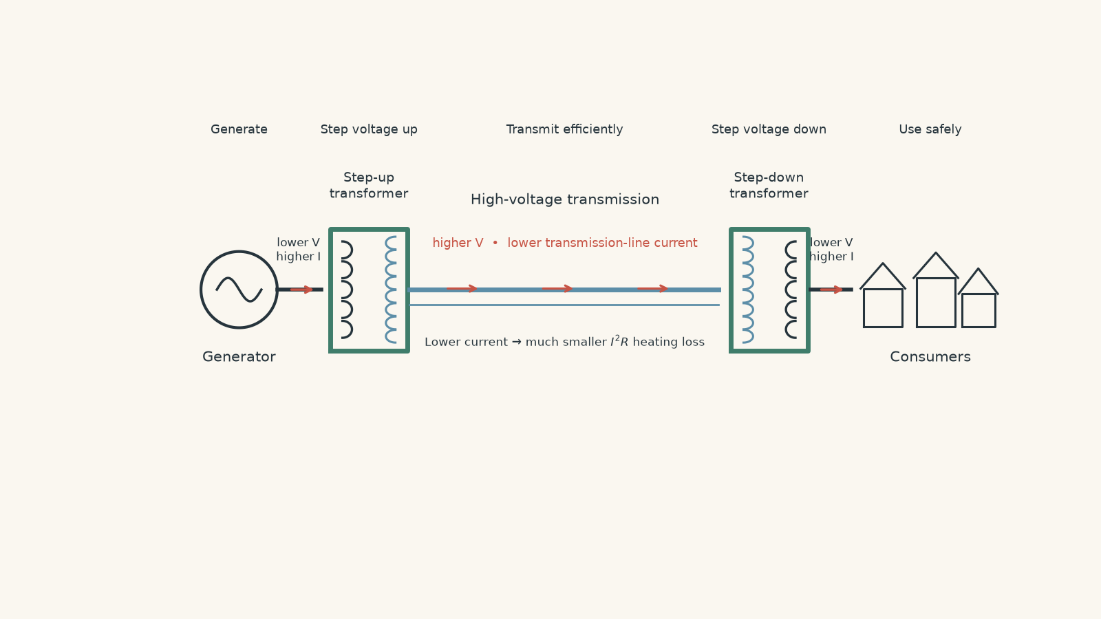
A step-up transformer increases the voltage before long-distance transmission. A step-down transformer later decreases the voltage for distribution and use.
For an ideal transformer,
\[ \frac{V_s}{V_p}=\frac{N_s}{N_p} \]
where:
- \(V_p\) is the primary voltage,
- \(V_s\) is the secondary voltage,
- \(N_p\) is the number of turns in the primary coil, and
- \(N_s\) is the number of turns in the secondary coil.
If the secondary coil has more turns than the primary coil, \(V_s>V_p\), so the transformer steps the voltage up.
The physical mechanism is electromagnetic induction. An alternating current in the primary coil produces a changing magnetic flux in the core. That changing flux induces an EMF in the secondary coil. If you need to revise the voltage and turns relationship in more detail, see tutorgum’s guide to the ideal transformer voltage and turns ratio.
An ideal transformer does not create power. Ignoring losses,
\[ P_p=P_s \]
so
\[ V_pI_p=V_sI_s \]
This gives the important trade-off.
If a transformer increases the voltage, it decreases the current.
For example, suppose an ideal transformer increases the voltage by a factor of 20. Its output current becomes one-twentieth of its input current.
That is exactly what we want before electricity enters a long transmission line.
03The transformer is not reducing the wire’s resistance
This misconception is worth dealing with directly.
A student might say:
“The transformer reduces energy loss because it makes the transmission line less resistive.”
It does not.
For a given line, its resistance is approximately determined by its material, length, cross-sectional area, and temperature. A transformer does not magically alter those properties kilometres away.
The chain of reasoning is instead
\[ \text{step up }V \rightarrow \text{lower }I\text{ for the same }P \rightarrow \text{lower }I^2R \rightarrow \text{less heating} \]
Keep those steps separate. That makes transmission questions much harder to get wrong.
Worked example: A step-up transformer before a transmission line
A generator supplies an ideal step-up transformer at \(11\ \text{kV}\) and \(50\ \text{A}\). The transformer has 20 times as many turns on its secondary coil as on its primary coil. The total resistance of the transmission line is \(16\ \Omega\).
Calculate the transmission voltage, the transmission current, and the power lost in the line. Then compare the line loss with the loss that would occur if the generator’s \(11\ \text{kV}\), \(50\ \text{A}\) output were sent directly through the same line.
Step 1
The turns ratio is
\[ \frac{N_s}{N_p}=20 \]
Therefore,
\[ \frac{V_s}{V_p}=20 \]
and
\[ V_s=20(11\ \text{kV})=220\ \text{kV} \]
Step 2
\[ P_p=V_pI_p =(11\times10^3)(50) =5.50\times10^5\ \text{W} \]
So the generator supplies \(550\ \text{kW}\).
For an ideal transformer, the secondary power is also \(550\ \text{kW}\).
Step 3
\[ I_s=\frac{P_s}{V_s} =\frac{5.50\times10^5}{220\times10^3} =2.5\ \text{A} \]
The transformer has increased the voltage by a factor of 20 and reduced the current by the same factor.
Step 4
\[ P_{\text{loss}} =I_s^2R =(2.5)^2(16) =100\ \text{W} \]
Only \(100\ \text{W}\) is converted to heat in the transmission line under this simplified ideal-transformer model.
Step 5
If the original \(50\ \text{A}\) current flowed through the same line,
\[ P_{\text{loss}} =(50)^2(16) =4.0\times10^4\ \text{W} =40\ \text{kW} \]
The step-up transformer reduced the current by a factor of 20, so the line loss fell by
\[ 20^2=400 \]
from \(40\ \text{kW}\) to \(0.100\ \text{kW}\).
The transformer has not supplied extra energy. It has changed the combination of voltage and current so that the same power can travel with far less resistive heating.
04Voltage drop improves too
Resistive heating is usually the main focus, but reducing current also reduces the voltage lost across the transmission line.
For a resistance \(R\),
\[ \Delta V=IR \]
where \(\Delta V\) is the potential difference across the line resistance.
Lower current therefore means both:
- less power converted to heat through \(P_{\text{loss}}=I^2R\), and
- a smaller voltage drop through \(\Delta V=IR\).
These relationships have different dependences on current. Halving \(I\) halves the voltage drop but quarters the resistive power loss.
05The equation that combines the whole argument
For a fixed transmitted power,
\[ I=\frac{P}{V} \]
Substitute this into
\[ P_{\text{loss}}=I^2R \]
to obtain
\[ P_{\text{loss}} = \left(\frac{P}{V}\right)^2R = \frac{P^2R}{V^2} \]
This equation makes the high-voltage advantage explicit:
\[ P_{\text{loss}}\propto\frac{1}{V^2} \]
provided the transmitted power \(P\) and line resistance \(R\) remain fixed.
That condition matters.
If the voltage doubles but the power being transmitted also doubles, then
\[ I=\frac{P}{V} \]
does not change. The line loss therefore does not change either.
So avoid memorising “double voltage means quarter loss” without the words for the same transmitted power.
06Real transformers are not ideal
The ideal-transformer model is useful because it exposes the basic transmission argument cleanly. Real transformers lose some energy.
Losses can include resistive heating in the coils and energy transferred to the transformer core. Eddy currents, for example, are unwanted currents induced within a conducting core. They cause heating and can be reduced by laminating the core. tutorgum has a separate guide on eddy-current losses in transformers if you are linking the transmission model to real transformer efficiency.
This adds an important layer of precision.
High voltage reduces losses in the transmission lines. It does not mean every other loss in the electricity system becomes zero.
A sensible transmission design therefore balances several effects. In an HSC calculation, use the model and data the question gives you rather than assuming every transformer is ideal.
07A compact method for HSC transmission questions
When you see a transformer and transmission-line problem, work through the physics in this order:
- Find the power being transmitted if it is not already given.
- Use the transformer ratio to find the transmission voltage, if required.
- Use \(P=VI\) to find the current in the transmission line.
- Use the line current, not automatically the generator current, in \(P_{\text{loss}}=I^2R\).
- If comparing systems, check what has been held constant: power, voltage, resistance, or some combination.
- Interpret the result physically. A smaller line current means less resistive heating.
A frequent exam error is to calculate the transformer’s secondary voltage correctly, then accidentally use the primary current in the line-loss calculation. Ask yourself one simple question: which current is actually flowing through the resistance named in the question?
08Questions and solutions
Question 1
A transmission line carries \(500\ \text{kW}\) at \(25\ \text{kV}\). The total resistance of the line is \(4.0\ \Omega\).
Calculate:
a. the current in the line, and
b. the power lost as heat in the line.
Solution 1
The line current is \(20\ \text{A}\), and the resistive power loss is \(1.6\ \text{kW}\).
First convert the power and voltage:
\[ P=500\times10^3\ \text{W} \]
\[ V=25\times10^3\ \text{V} \]
Using
\[ P=VI \]
gives
\[ I=\frac{P}{V} =\frac{500\times10^3}{25\times10^3} =20\ \text{A} \]
For the line loss,
\[ P_{\text{loss}}=I^2R =(20)^2(4.0) =1600\ \text{W} \]
Therefore,
\[ P_{\text{loss}}=1.6\ \text{kW} \]
The tempting mistake is to substitute the transmission voltage into a resistance-power formula without first finding the line current. The relevant heating relationship here is \(I^2R\): it is the current through the line resistance that determines the loss.
Question 2
A system transmits \(6.6\ \text{MW}\) through a line with total resistance \(12\ \Omega\).
Compare the line loss when the transmission voltage is:
a. \(33\ \text{kV}\), and
b. \(132\ \text{kV}\).
By what factor has the loss changed?
Solution 2
The losses are \(480\ \text{kW}\) at \(33\ \text{kV}\) and \(30\ \text{kW}\) at \(132\ \text{kV}\). Increasing the voltage by a factor of four reduces the line loss to one-sixteenth.
At \(33\ \text{kV}\),
\[ I=\frac{P}{V} =\frac{6.6\times10^6}{33\times10^3} =200\ \text{A} \]
Therefore,
\[ P_{\text{loss}} =(200)^2(12) =4.8\times10^5\ \text{W} =480\ \text{kW} \]
At \(132\ \text{kV}\),
\[ I=\frac{6.6\times10^6}{132\times10^3} =50\ \text{A} \]
so
\[ P_{\text{loss}} =(50)^2(12) =3.0\times10^4\ \text{W} =30\ \text{kW} \]
The voltage has increased by
\[ \frac{132}{33}=4 \]
while the current has fallen by a factor of four.
Because the loss depends on the square of current,
\[ \frac{P_{\text{loss,new}}}{P_{\text{loss,old}}} = \left(\frac{1}{4}\right)^2 = \frac{1}{16} \]
A student might predict that four times the voltage gives one-quarter of the loss. That would be true for a quantity proportional directly to current. Resistive heating depends on \(I^2\), so the improvement is squared.
Question 3
A power station supplies \(2.00\ \text{MW}\) to a step-up transformer whose primary voltage is \(10.0\ \text{kV}\). The transformer increases the voltage to \(200\ \text{kV}\) and is \(98.0\%\) efficient.
The transmission line has a total resistance of \(50.0\ \Omega\).
a. Calculate the power delivered to the transmission line by the transformer.
b. Calculate the current in the transmission line.
c. Calculate the power lost in the transmission line.
d. A student says, “Because the transformer is only \(98\%\) efficient, it must also make the line heating \(2\%\) larger than it would be for an ideal transformer.” Explain whether this is correct.
Solution 3
The transformer delivers \(1.96\ \text{MW}\) to the line, the transmission current is \(9.80\ \text{A}\), and the line loses about \(4.80\ \text{kW}\). The student’s claim is incorrect: the inefficient transformer slightly reduces the power reaching the line and therefore slightly reduces the line current, although it increases the total losses of the complete system.
For the transformer,
\[ \eta=\frac{P_{\text{out}}}{P_{\text{in}}} \]
where \(\eta\) is the efficiency.
Therefore,
\[ P_{\text{out}} =\eta P_{\text{in}} =(0.980)(2.00\times10^6) =1.96\times10^6\ \text{W} \]
So the transformer supplies
\[ P_{\text{out}}=1.96\ \text{MW} \]
to the transmission line.
The line current is
\[ I=\frac{P}{V} =\frac{1.96\times10^6}{200\times10^3} =9.80\ \text{A} \]
The line loss is therefore
\[ P_{\text{loss}} =I^2R =(9.80)^2(50.0) =4.802\times10^3\ \text{W} \]
or approximately
\[ P_{\text{loss}}=4.80\ \text{kW} \]
For comparison, an ideal transformer would deliver the full \(2.00\ \text{MW}\) at \(200\ \text{kV}\), giving
\[ I_{\text{ideal}} =\frac{2.00\times10^6}{200\times10^3} =10.0\ \text{A} \]
and
\[ P_{\text{loss,ideal}} =(10.0)^2(50.0) =5.00\ \text{kW} \]
So the real transformer actually produces slightly less line heating because less power reaches the line.
That does not make inefficiency beneficial. The transformer itself loses
\[ 2.00\ \text{MW}-1.96\ \text{MW} =40.0\ \text{kW} \]
before the line is even reached.
The trap is to treat “loss” as if all losses occur in one place. Transformer losses and transmission-line losses are separate energy transfers and must be calculated separately.
Question 4
A simplified system must transmit \(1.00\ \text{MW}\).
Design A sends the power directly at \(10.0\ \text{kV}\).
Design B uses transformers to transmit at \(100\ \text{kV}\). At this operating point, the two transformers together dissipate \(10.0\ \text{kW}\). Treat this transformer loss as given. Both designs use a transmission line with the same total resistance \(R\).
Ignore the small change in transmitted power caused by line losses when calculating current.
a. Find the value of \(R\) at which the total power loss of the two designs is equal.
b. Which design has the smaller total loss when \(R=0.50\ \Omega\)?
c. Explain why this does not contradict the rule that high voltage reduces transmission-line losses.
Solution 4
The two designs have equal total loss when \(R\approx1.01\ \Omega\). At \(R=0.50\ \Omega\), the direct \(10.0\ \text{kV}\) design has the smaller total loss. There is no contradiction because high voltage always reduces the resistive line loss under these conditions, but Design B also contains an additional transformer loss.
For Design A,
\[ I_A=\frac{1.00\times10^6}{10.0\times10^3} =100\ \text{A} \]
Its total loss is simply its line loss:
\[ P_{\text{loss,A}} =I_A^2R =(100)^2R =10000R \]
For Design B,
\[ I_B=\frac{1.00\times10^6}{100\times10^3} =10.0\ \text{A} \]
Its line loss is
\[ P_{\text{line,B}} =(10.0)^2R =100R \]
But Design B also has \(10.0\ \text{kW}=10000\ \text{W}\) of transformer loss, so
\[ P_{\text{loss,B}}=100R+10000 \]
For equal total losses,
\[ 10000R=100R+10000 \]
so
\[ 9900R=10000 \]
and
\[ R=\frac{10000}{9900} \approx1.01\ \Omega \]
Now take \(R=0.50\ \Omega\).
For Design A,
\[ P_{\text{loss,A}} =10000(0.50) =5000\ \text{W} =5.00\ \text{kW} \]
For Design B,
\[ P_{\text{loss,B}} =100(0.50)+10000 =10050\ \text{W} =10.05\ \text{kW} \]
So Design A loses less power in this particular case.
The tempting route is to say, “\(100\ \text{kV}\) is ten times \(10\ \text{kV}\), so Design B must always be better.” Its line loss is indeed 100 times smaller:
\[ 100R \quad\text{instead of}\quad 10000R \]
But the question asks about total loss. When the line resistance is small enough, the \(10.0\ \text{kW}\) transformer loss is larger than the line energy saved.
This is a boundary case worth remembering. High transmission voltage reduces \(I^2R\) losses in the line. It does not prove that every imaginable high-voltage system has lower total losses once other components are included.
Question 5
A transmission network carries power from one station to two towns, A and B.
A shared transmission line runs from the station to a junction and has resistance \(6.0\ \Omega\). From the junction, separate lines run to towns A and B. Each branch has resistance \(4.0\ \Omega\).
Each branch carries \(3.30\ \text{MW}\). Initially, the shared line and both branches operate at \(132\ \text{kV}\).
Assume ideal transformers and ignore the small effect of line losses when calculating the transmitted currents.
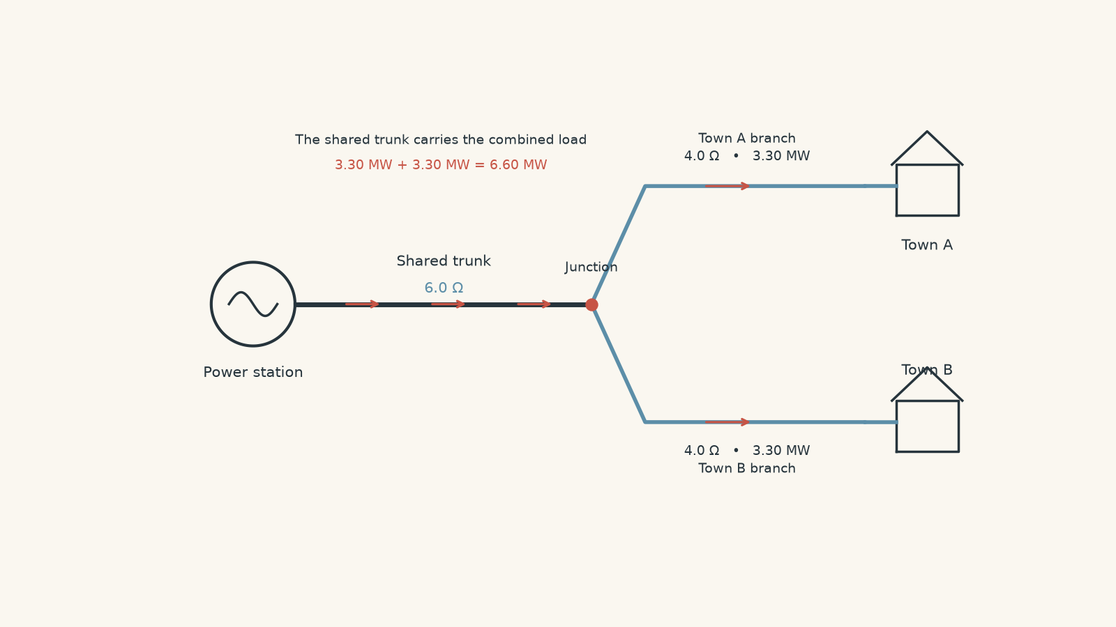
a. Calculate the total resistive line loss in the original network.
An engineer then installs an ideal step-up transformer at the junction so that only the line from the junction to Town B operates at \(264\ \text{kV}\). An ideal step-down transformer at Town B returns the voltage to the required level.
b. Calculate the new total line loss.
A student argues that because Town B’s branch current has halved, Town B’s contribution to the current in the shared line must also halve.
c. Explain the error.
Finally, instead of upgrading only Town B’s branch, suppose the entire transmission network – shared line and both branches – operates at \(264\ \text{kV}\).
d. Calculate the total line loss in this case and explain why this result differs so much from upgrading only the Town B branch.
Solution 5
The original network loses \(20.0\ \text{kW}\). Raising only Town B’s branch to \(264\ \text{kV}\) reduces the total loss only to \(18.125\ \text{kW}\), because the shared line still operates at \(132\ \text{kV}\) and still carries the power for both towns. Raising the entire network to \(264\ \text{kV}\) reduces the total line loss to \(5.00\ \text{kW}\), exactly one-quarter of the original value.
Start with one branch.
At \(132\ \text{kV}\),
\[ I_{\text{branch}} =\frac{P}{V} =\frac{3.30\times10^6}{132\times10^3} =25.0\ \text{A} \]
Both branches carry \(25.0\ \text{A}\).
Before the current reaches the junction, the shared line must carry power for both towns. Its current is therefore
\[ I_{\text{shared}} =25.0+25.0 =50.0\ \text{A} \]
The shared-line loss is
\[ P_{\text{shared}} =(50.0)^2(6.0) =15000\ \text{W} =15.0\ \text{kW} \]
Each branch loses
\[ P_{\text{branch}} =(25.0)^2(4.0) =2500\ \text{W} =2.50\ \text{kW} \]
There are two branches, so the original total loss is
\[ P_{\text{total}} =15.0+2.50+2.50 =20.0\ \text{kW} \]
Now raise only Town B’s branch voltage to \(264\ \text{kV}\).
Its current becomes
\[ I_B =\frac{3.30\times10^6}{264\times10^3} =12.5\ \text{A} \]
So the Town B branch loss becomes
\[ P_B =(12.5)^2(4.0) =625\ \text{W} =0.625\ \text{kW} \]
Town A’s branch has not changed, so its loss remains \(2.50\ \text{kW}\).
The crucial step is the shared line.
The step-up transformer for Town B is at the junction. Upstream of that transformer, the shared line is still at \(132\ \text{kV}\). An ideal transformer changes voltage and current on opposite sides of itself, but it does not remove the power that has to reach Town B.
Town B still requires \(3.30\ \text{MW}\). At \(132\ \text{kV}\), supplying that power to the transformer’s input requires
\[ I=\frac{3.30\times10^6}{132\times10^3} =25.0\ \text{A} \]
So Town B still contributes \(25.0\ \text{A}\) to the shared-line current before the transformer.
The shared current therefore remains
\[ I_{\text{shared}}=25.0+25.0=50.0\ \text{A} \]
and the shared-line loss remains \(15.0\ \text{kW}\).
The new total is
\[ P_{\text{total}} =15.0+2.50+0.625 =18.125\ \text{kW} \]
The student’s mistake is subtle. They have treated the \(12.5\ \text{A}\) current on the transformer’s high-voltage side as though that same current must exist on its low-voltage side.
It does not.
The transformer changes the current at the junction. The location of the transformer matters. A reduction in current downstream of the transformer does not travel backwards through the circuit as the same numerical current.
Now consider raising the entire network to \(264\ \text{kV}\).
Each branch current is now
\[ I_{\text{branch}}=12.5\ \text{A} \]
so the shared line carries
\[ I_{\text{shared}} =12.5+12.5 =25.0\ \text{A} \]
Its loss is
\[ P_{\text{shared}} =(25.0)^2(6.0) =3750\ \text{W} =3.75\ \text{kW} \]
Each branch loses
\[ P_{\text{branch}} =(12.5)^2(4.0) =625\ \text{W} =0.625\ \text{kW} \]
Therefore,
\[ P_{\text{total}} =3.75+0.625+0.625 =5.00\ \text{kW} \]
The entire network voltage has doubled while its transmitted powers and resistances have stayed fixed. Every relevant current has therefore halved, so every \(I^2R\) loss has been quartered:
\[ \frac{20.0\ \text{kW}}{4}=5.00\ \text{kW} \]
This is the important hinge in the problem: saying “higher voltage gives lower current” is not enough. You must ask where the higher voltage exists.
A transformer only reduces the current in the part of the network on its high-voltage side. To work out which resistive losses fall, trace the actual current path and locate the transformer before applying \(I^2R\).
09What this idea unlocks next
High-voltage transmission is really an application of two linked principles: power can be transferred using different combinations of voltage and current, and resistive heating depends on the square of current.
Transformers make that trade possible in an AC grid. They step the voltage up before a long resistive path, allowing the required power to travel at low current, then step the voltage down again where lower voltages are needed.
Once that picture is secure, the next useful question is no longer simply “Why use high voltage?” It becomes: how close can a real transformer get to the ideal behaviour assumed in these calculations, and where does the missing energy go? That leads directly into transformer efficiency, coil heating, eddy currents, incomplete flux linkage, and the other limits that separate the ideal model from a real electricity grid.