
How to Evaluate Accuracy, Reliability and Validity in HSC Physics
Learn how to evaluate accuracy, reliability, and validity in HSC Physics practicals using actual measurements, graphs, experimental controls, and specific limitations. Includes worked examples on gravitational acceleration, circuit relationships, and refractive index, plus sentence frameworks and challenging practice questions with solutions.
Imagine two groups measuring gravitational acceleration, \(g\). One group gets almost the same value every time, but its mean is far from the accepted value. The other group’s mean is closer to the accepted value, but its measurements vary widely. Which group’s practical is better?
The first group has more consistent measurements. The second may have a more accurate mean. But neither result tells you, by itself, whether the method validly tested the relationship between height and falling time.
This is the key to evaluating an HSC Physics practical: accuracy, reliability, and validity describe different things, so you need different evidence to support each claim.
- Accuracy: How close is the measured result to an appropriate reference value?
- Reliability: How consistent are repeated measurements?
- Validity: Does the method actually test the intended question, with other relevant factors controlled?
A strong evaluation connects each judgement to measurements, a graph, an experimental control, or a specific limitation. Simply writing that human error affected the results will not do the job.
Three different ways to evaluate a physics practical
| Accuracy | Compare the measured result with an accepted reference value. How close is your result to the reference? |
|---|---|
| Reliability | Repeated measurements cluster closely, showing a small spread. How consistent are your repeated results? |
| Validity | Control relevant variables while testing the intended relationship. Does your method test what you intended to investigate? |
01Accuracy, reliability, and validity are not interchangeable
Accuracy: compare your result with a reference
Accuracy describes how close an experimental measurement or calculated result is to its true value. In practice, you usually assess it by comparing your result with an accepted or independently established reference value.
For example, when measuring gravitational acceleration near Earth’s surface, a commonly used reference is approximately \(9.8\ \mathrm{m\,s^{-2}}\). You would compare your experimentally determined value of \(g\) with the appropriate reference value.
For a numerical comparison, calculate the percentage error:
\[ \%\text{ error} = \frac{|x_{\text{measured}}-x_{\text{reference}}|} {|x_{\text{reference}}|} \times 100\% \]
Here, \(x_{\text{measured}}\) is your experimental result and \(x_{\text{reference}}\) is the accepted value of the same quantity.
A smaller percentage error indicates closer agreement with the reference. However, check that the reference applies to the same material, conditions, and quantity you measured.
You also need to consider measurement uncertainty. A small difference from a reference may not be significant if it is comparable to the uncertainty in your result.
What counts as evidence of accuracy?
- A measured value compared with an appropriate reference.
- A calculated percentage error.
- An estimate of uncertainty, where available.
- Evidence that the instruments were suitable and correctly calibrated.
A straight-line graph does not automatically establish accuracy. A graph can follow the expected pattern while its gradient is systematically too large or too small.
If you have no suitable reference value, you can discuss possible sources of error and the quality of your method. You should not claim to have demonstrated high accuracy without enough evidence to support that conclusion.
Reliability: examine repeated measurements
Reliability describes the consistency of repeated measurements made under the same conditions.
Suppose you measure the time taken for an object to fall from the same height several times. If the recorded times are tightly clustered, this supports the reliability of the timing procedure.
One simple measure of spread is the range:
\[ \text{Range}=x_{\max}-x_{\min} \]
Here, \(x_{\max}\) and \(x_{\min}\) are the largest and smallest recorded values.
The range gives you something concrete to discuss. You can report the actual spread in your measurements and explain what it suggests about repeatability.
However, the range is not enough on its own. Consider the size of the spread relative to the measured quantity and the instrument’s resolution.
What counts as evidence of reliability?
- Repeated trials under the same conditions.
- The range or spread of repeated measurements.
- Similar results when the procedure is repeated.
- Consistent patterns across repeated measurements or independently repeated runs.
One important trap: a group can obtain very consistent results that are all systematically wrong.
For example, if a timer consistently records a falling object’s time as too long, repeating the measurement will not remove that bias. The readings may be reliable but inaccurate.
More trials help you identify random variation and estimate a mean more reliably. They do not automatically remove a systematic error.
Validity: check whether the method tests the right thing
Validity concerns whether your experimental method and evidence allow you to answer the intended research question.
In an investigation of a relationship between two variables, you need to change the independent variable, measure the dependent variable appropriately, and control other factors that could influence the result.
Consider testing the relationship between potential difference and current through a metallic resistor. If the resistor heats up significantly as the current increases, its resistance may change. You are no longer testing the relationship under a constant-temperature condition.
The measurements could be highly repeatable. They could even look reasonably close to a predicted relationship over part of the range. But an uncontrolled temperature change weakens the validity of the investigation if the intended model assumes constant resistance.
What counts as evidence of validity?
- Appropriate control of relevant variables.
- A method that measures the intended quantities.
- A suitable range of independent-variable values.
- Instruments and procedures capable of testing the proposed relationship.
- Evidence that alternative explanations have been considered.
A valid method does not need to be perfect. It needs to be suitable for answering the question, and its limitations need to be recognised when interpreting the evidence.
Keep the three judgements separate
| Criterion | Main evidence | A claim you should avoid |
|---|---|---|
| Accuracy | Comparison with a suitable reference | “The results were close together, so they were accurate.” |
| Reliability | Spread of repeated measurements | “The mean was close to the reference, so the experiment was reliable.” |
| Validity | Controls, measurement method, and suitability of the investigation | “The graph was straight, so the experiment was valid.” |
Evaluate a physics practical using three separate checks
- Check accuracy
Is a suitable reference value available? Compare it with the measured result.
- Check reliability
Examine the spread of repeated measurements; a smaller spread indicates greater consistency.
- Check validity
Were relevant variables controlled and the intended quantities measured?
02Turn a limitation into an explanation
A practical evaluation is not a list of things that might have gone wrong. It is an argument about how the method could have affected the evidence.
Use this chain:
Specific limitation → physical mechanism → effect on measurements or graph → consequence for the conclusion → improvement.
Each link matters. Naming a limitation without explaining its effect does not tell the reader whether it matters, or how.
For example, compare these two statements.
Weak:
Human error may have affected the timing.
Stronger:
If the start and stop delays made the recorded fall times systematically longer, the calculated gravitational acceleration would be underestimated because \(g=2h/t^2\). Using video-frame timing or an appropriate electronic timing system would reduce the dependence on human reaction time.
The stronger statement identifies the limitation, explains the mathematical consequence, and proposes an improvement that addresses the actual problem.
Notice the word if. Unless you have evidence that the measured times were systematically too long, you should not claim that this definitely happened in your experiment.
A sentence framework you can adapt
Build a strong experimental evaluation
- Identify the limitation
Name a specific weakness in the method.
- Explain the mechanism
Describe how the limitation affects the measurement.
- Identify affected evidence
Name the measurement, calculated result or graph feature.
- Assess the consequence
Explain how the conclusion may be affected; qualify uncertainty.
- Target an improvement
Propose a change that reduces the identified mechanism.
Use the following frameworks with the measurements and observations from your own practical.
For accuracy:
“The experimentally determined value of ___ was ___ [unit], compared with the reference value of ___ [unit]. The percentage error was ___%. This indicates ___ agreement with the reference, although ___ must be considered when interpreting the difference.”
For reliability:
“The repeated measurements of ___ ranged from ___ to ___ [unit], giving a range of ___. This indicates ___ consistency under the experimental conditions. However, the spread does not establish whether the result was accurate because ___.”
For validity:
“The investigation varied ___ to test its relationship with ___, while ___ was controlled by ___. However, ___ may have changed ___, which could have affected ___. Therefore, the evidence ___ the proposed relationship, subject to this limitation.”
For a specific limitation:
“Because ___, the measured ___ could ___. This would cause ___ in the calculated result or graph because ___. The effect on the conclusion is ___. To reduce this limitation, ___.”
The final part of the sentence should follow from the mechanism. If you cannot establish whether a limitation makes a result too high or too low, say that it could increase uncertainty or bias the result in either direction. Do not guess.
03Worked example: measuring gravitational acceleration
Worked example: evaluating a free-fall experiment
A class estimates gravitational acceleration by dropping a dense ball from several measured heights. At each height, students repeat the timing, calculate a mean time, and plot height \(h\) against the square of the mean time, \(t^2\). Explain how they should evaluate accuracy, reliability, and validity without assuming what their experimental results show.
Step 1
For an object released from rest and falling with negligible air resistance, the displacement is
\[ h=\frac{1}{2}gt^2 \]
Here:
- \(h\) is the vertical displacement in metres (\(\mathrm{m}\)).
- \(g\) is gravitational acceleration in \(\mathrm{m\,s^{-2}}\).
- \(t\) is the elapsed time in seconds (\(\mathrm{s}\)).
Rearranging gives
\[ g=\frac{2h}{t^2} \]
This equation provides a way to calculate \(g\) from a measured height and fall time. It also predicts that a graph of \(h\) against \(t^2\) should be linear if the model’s assumptions hold.
Step 2
For a graph with \(h\) on the vertical axis and \(t^2\) on the horizontal axis, the gradient is
\[ m=\frac{\Delta h}{\Delta(t^2)} \]
Comparing this with \(h=\frac12gt^2\) gives
\[ m=\frac{g}{2} \]
Therefore,
\[ g_{\text{exp}}=2m \]
The gradient has units of \(\mathrm{m\,s^{-2}}\), so the calculated value of \(g\) has the correct units.
Substitute the gradient measured from your own graph:
\[ g_{\text{exp}}=2 \left[\text{measured gradient in }\mathrm{m\,s^{-2}}\right] \]
This gives the experimental value without assuming a gradient that was never measured.
Step 3
For each fixed height, compare the repeated fall times. Calculate the range using the largest and smallest recorded times.
A small spread relative to the measurement resolution supports consistent timing. A large spread suggests that the timing procedure is not producing consistent measurements.
If the class used manual timing, reaction-time variation is one possible explanation. However, the measurements themselves must support the claim that the timing was inconsistent.
Step 4
Compare the experimental value of \(g\), calculated from the graph’s gradient, with an appropriate accepted value.
\[ \%\text{ error} = \frac{|g_{\text{exp}}-g_{\text{ref}}|} {|g_{\text{ref}}|} \times100\% \]
Here, \(g_{\text{ref}}\) is the reference gravitational acceleration.
A small percentage error indicates close agreement. A large percentage error indicates a substantial difference, although the estimated uncertainty should also be considered.
A straight graph does not establish accuracy. The gradient could be biased even when the points follow a clear linear pattern.
Step 5
The model assumes that the object starts from rest, that the measured height represents its vertical displacement, and that air resistance is negligible.
A push during release changes the initial velocity, so the equation \(h=\frac12gt^2\) no longer describes the motion as written. An inconsistent reference point for measuring height can also distort the relationship between recorded height and elapsed time.
A suitable improvement would be to use a consistent release method and a clearly defined height reference. Electronic timing or video analysis may reduce reaction-time effects.
The final evaluation should distinguish between the evidence for repeatability, the comparison with the accepted value, and the extent to which the method satisfies the assumptions of the model.
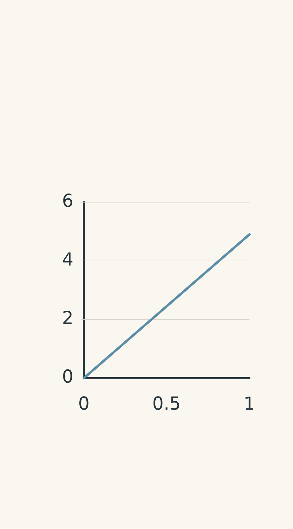
- Straight best-fit line: gradient = g/2; g = 2 × gradient
04Worked example: testing a circuit relationship
Worked example: evaluating potential difference against current
A student investigates whether the potential difference across a fixed metallic resistor is proportional to the current through it. They vary the electrical conditions, record potential difference \(V\) and current \(I\), and plot \(V\) against \(I\). Explain how the student should evaluate the relationship and the quality of the practical.
Step 1
For a resistor obeying Ohm’s law under constant physical conditions,
\[ V=IR \]
where:
- \(V\) is potential difference in volts (\(\mathrm{V}\)).
- \(I\) is current in amperes (\(\mathrm{A}\)).
- \(R\) is resistance in ohms (\(\Omega\)).
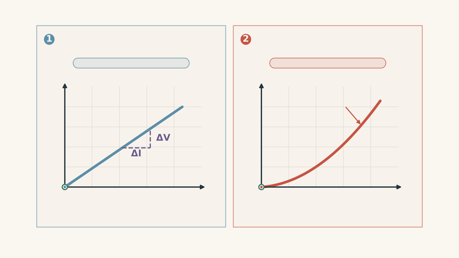
If resistance remains constant, potential difference is proportional to current. A graph of \(V\) against \(I\) should be linear and pass through the origin, within experimental uncertainty.
Step 2
For a straight-line graph of \(V\) against \(I\),
\[ R=m=\frac{\Delta V}{\Delta I} \]
The units are
\[ \frac{\mathrm{V}}{\mathrm{A}}=\Omega \]
Substitute the gradient calculated from the student’s actual graph:
\[ R= \frac{\text{change in measured }V} {\text{change in measured }I} \]
This produces an experimental resistance. No numerical resistance should be reported until the actual measurements or graph gradient are available.
Step 3
If the student repeated measurements at the same settings, compare the repeated voltage and current readings. A small spread supports repeatability.
If only one reading was taken at each setting, the overall graph may show a consistent trend, but this does not provide the same evidence of repeatability as repeated trials.
Step 4
A metallic resistor can heat up as current increases. Its resistance then generally increases with temperature.
This creates an important problem. If the aim is to test whether \(V\) is proportional to \(I\) at constant temperature, allowing the resistor to heat substantially introduces another changing factor.
The graph may become curved, with an increasing gradient. Treating the entire graph as a single constant resistance could then be misleading.
A suitable improvement is to limit heating, allow the resistor to cool between measurements where appropriate, and keep its temperature as constant as practicable.
Step 5
If an appropriate reference resistance is available, compare it with the experimental resistance calculated from the graph.
A close match supports accuracy for that comparison. It does not, by itself, demonstrate that temperature was controlled or that the full investigation was valid.
Likewise, a repeatable set of voltage and current readings does not prove that resistance remained constant.
05Applying the same reasoning to refractive index
Refraction provides a useful third example because a practical can produce a clear mathematical relationship while still containing systematic errors.
When light passes from air into a transparent material, its direction changes. The relationship between the angle of incidence and the angle of refraction is described by Snell’s law:
\[ n_1\sin i=n_2\sin r \]
Here, \(n_1\) and \(n_2\) are the refractive indices of the two media, \(i\) is the angle of incidence, and \(r\) is the angle of refraction. Both angles are measured from the normal, which is perpendicular to the surface.
For light travelling from air into a transparent block, taking the refractive index of air as approximately 1 gives
\[ n\approx\frac{\sin i}{\sin r} \]
where \(n\) is the refractive index of the block.
Worked example: evaluating a refractive-index investigation
A student traces light through a transparent block, measures several pairs of incidence and refraction angles, and plots \(\sin i\) against \(\sin r\). Explain how to use the graph and evaluate the method without assuming any particular experimental result.
Step 1
If \(\sin i\) is on the vertical axis and \(\sin r\) is on the horizontal axis, then
\[ \sin i=n\sin r \]
The gradient is therefore
\[ m=\frac{\Delta(\sin i)}{\Delta(\sin r)} \]
For light entering the block from air,
\[ n\approx m \]
The gradient is dimensionless because both sine values are dimensionless.
Use the gradient from the actual graph to determine the experimental refractive index. A linear trend supports the predicted relationship, but it does not independently establish accuracy.
Step 2
If the student repeats the angle measurements or traces the same paths again, compare the resulting angle pairs or calculated refractive indices.
A small spread supports repeatability. A large spread suggests that tracing, alignment, or angle measurement may be inconsistent.
If only one reading is taken at each incidence angle, the spread between different angles should not automatically be described as poor reliability. The measurements represent different experimental conditions. Repeated measurements at the same condition provide clearer evidence of repeatability.
Step 3
Compare the experimental refractive index with an appropriate reference value for the same material and relevant conditions.
Wavelength matters because a material’s refractive index can vary with the wavelength of light. Temperature and material composition may also matter.
Comparing a result with a reference value for a different wavelength may therefore produce a difference that cannot be attributed solely to experimental error.
Step 4
Both angles must be measured from the normal, not from the surface. If the student measures angles from the surface but substitutes them into Snell’s law as though they were measured from the normal, the calculated refractive index will be incorrect.
Using several incidence angles helps test the predicted relationship across a range. The same material and light wavelength should be maintained throughout the investigation.
Thick traced lines can make the exact light path uncertain, increasing the uncertainty in the measured angles. Drawing finer lines and repeating measurements can help, but they cannot correct a consistently misdrawn normal.
The key point is that accuracy, reliability, and validity require different evidence even when they concern the same refractive-index experiment.
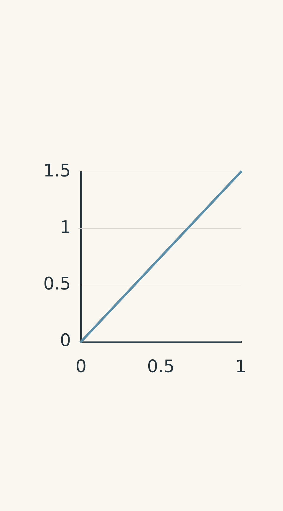
- Schematic best-fit line through origin; gradient = n
06Common limitations and their likely effects
Use the following examples to connect a limitation to its mechanism and the evidence it may affect.
| Practical | Specific limitation | Likely effect on the evidence | Targeted improvement |
|---|---|---|---|
| Measuring \(g\) | Manual timing introduces a consistent positive time bias. | If measured time is too long, \(g=2h/t^2\) is underestimated. | Use suitable electronic timing or video analysis. |
| Measuring \(g\) | The object receives a push at release. | The initial velocity is no longer zero, so the assumed free-fall equation does not apply as written. | Use a consistent release mechanism. |
| Testing a circuit relationship | A metallic resistor heats as current increases. | Resistance changes, potentially producing a changing gradient in the \(V\)-against-\(I\) graph. | Reduce heating and control temperature. |
| Determining refractive index | The normal is drawn incorrectly. | Both angle measurements may be systematically biased, shifting the calculated ratio or graph gradient. | Establish the perpendicular reference accurately. |
| Determining refractive index | Thick ray-tracing lines make the path difficult to locate. | Angle uncertainty increases, potentially increasing scatter in the calculated refractive indices. | Use finer lines and repeat measurements. |
The effect must be justified. For example, a timing bias that makes every measured time longer has a predictable direction of effect on the calculated \(g\). A poorly drawn normal, on the other hand, may bias the refractive-index result in either direction, depending on the geometry.
Do not force a directional claim when the available evidence does not establish one.
Random and systematic errors
These terms help you explain why a limitation matters.
Random errors cause measurements to vary unpredictably. Examples include variation in manual reaction time and uncertainty in locating the centre of a thick traced line. They can increase the spread of repeated measurements.
Systematic errors shift measurements consistently in one direction. Examples include a timer that consistently records an extra delay or a misaligned reference used for every angle measurement. They can bias the calculated result even when repeated readings agree closely.
Repeating measurements can help reduce the influence of random variation on a mean. Repetition alone does not remove a fixed systematic bias.
A systematic error may also affect validity if it means the procedure no longer measures the intended quantity correctly. The exact consequence depends on the investigation and how the data are analysed.
07Write conclusions that match the evidence
Before submitting your evaluation, check what your data actually allow you to say.
| If your evidence shows… | A defensible conclusion is… |
|---|---|
| Repeated readings have a small spread. | The measurements show good repeatability under the conditions tested. |
| The experimental result is close to a suitable reference. | The result shows close agreement with the reference, subject to uncertainty. |
| A graph follows the predicted relationship. | The observed pattern is consistent with the model over the tested range. |
| A relevant variable was not controlled. | The uncontrolled variable may have influenced the measurements and weakened the validity of the conclusion. |
| No suitable reference value is available. | Accuracy cannot be quantified from the available evidence alone. |
| Only one reading was taken at each setting. | The graph shows the pattern across the tested settings, but repeatability has not been established by repeated readings at each setting. |
The final row is especially useful. A graph made from many points can look convincing, but the number of points alone does not establish reliability. Likewise, a small percentage error cannot prove that every experimental control was appropriate.
A strong evaluation also avoids claiming that an improvement will solve every problem. Video timing may reduce reaction-time effects in a free-fall experiment, for example, but it will not automatically correct a mismeasured height or an unsuitable motion model.
08Questions and solutions
Question 1
A student repeats a measurement five times. The results are tightly clustered, but the student has not compared the mean with an accepted reference value.
Can the student conclude that the result is accurate and reliable? Explain which claims are supported by the evidence.
Solution 1
The evidence supports reliability, but it is not sufficient to establish accuracy.
The tightly clustered measurements indicate that repeated trials produced similar results under the conditions used. This is evidence of repeatability.
Accuracy requires a comparison with an appropriate reference value, or other evidence capable of establishing closeness to the true value. Without that comparison, the student cannot confidently claim high accuracy.
The student should also consider validity separately by checking whether the method measured the intended quantity and controlled relevant variables. Consistent measurements do not guarantee a suitable method.
Question 2
A student estimates gravitational acceleration using
\[ g=\frac{2h}{t^2} \]
The student’s timing system consistently records a fall time that is longer than the actual time by a positive amount \(\delta\). Assume the measured height is correct and air resistance is negligible.
Explain how this affects the calculated value of \(g\). Would repeating the measurement remove the problem?
Solution 2
The calculated gravitational acceleration will be underestimated, and repeating the measurement will not remove the consistent timing bias.
Let the actual fall time be \(t\). The measured time is
\[ t_{\text{measured}}=t+\delta \]
where \(\delta>0\).
Substituting the measured time into the calculation gives
\[ g_{\text{measured}} =\frac{2h}{(t+\delta)^2} \]
Since \(\delta\) is positive,
\[ (t+\delta)^2>t^2 \]
The denominator is therefore larger than it should be. With the height unchanged, the calculated value of \(g\) is smaller than the value obtained using the actual fall time.
The readings may still be reliable if the timing bias is consistent and the repeated measurements have little spread. However, the systematic bias reduces accuracy.
The timing method also weakens the validity of the calculation because the recorded time does not represent the true elapsed time. Repeating the same measurement may reduce random variation, but it will not eliminate the fixed delay. A suitable electronic timing method or video analysis could reduce this limitation.
Question 3
A student tests the relationship between potential difference and current through a metallic resistor. At higher currents, the resistor becomes warmer. Repeated measurements at each setting are consistent, but the \(V\)-against-\(I\) graph begins to curve.
Can the student conclude that Ohm’s law holds across the entire tested range? Explain how the temperature change affects the evaluation.
Solution 3
No. The student cannot conclude that the constant-resistance relationship holds across the entire range because the changing temperature may be changing the resistance.
For a resistor with constant resistance,
\[ V=IR \]
A graph of \(V\) against \(I\) should be linear, with a constant gradient equal to the resistance.
For a metallic resistor, increasing temperature generally increases resistance. The gradient of the \(V\)-against-\(I\) graph can therefore increase as the current increases, producing a curved relationship.
The consistent repeated measurements support reliability, but they do not establish validity. The temperature change introduces another factor that affects the relationship being investigated.
To improve the investigation, the student should reduce heating and maintain a more consistent resistor temperature. If the aim is to test Ohm’s law under constant-temperature conditions, the conclusion should be based on evidence gathered under those conditions rather than treating the entire curved graph as one constant resistance.
Question 4
A student determines the refractive index of a transparent material and obtains an experimental value that differs from a published reference value. The reference is for the same material but a different wavelength of light.
The student concludes that the practical was inaccurate. Evaluate this conclusion and identify the evidence needed for a more defensible judgement.
Solution 4
The difference alone does not establish that the practical was inaccurate because the reference value was determined under different optical conditions.
A material’s refractive index can depend on wavelength. The student’s experimental value and the published reference may therefore differ even if both are reasonable measurements for their respective conditions.
For a meaningful accuracy assessment, the student should compare the experimental result with a reference value for the same material and an appropriate matching wavelength. Other relevant conditions should also be considered.
Reliability should be evaluated using repeated angle measurements or repeated calculated refractive indices at the same experimental conditions. A small spread would support repeatability.
Validity requires checking that both incidence and refraction angles were measured from the normal, that the same material was used, and that the wavelength remained constant throughout the investigation.
A graph consistent with Snell’s law supports the predicted relationship. It does not, by itself, establish accuracy or rule out systematic errors in the angle measurements.
Question 5
A class measures gravitational acceleration using free fall. The actual displacement \(h\) and elapsed time \(t\) obey
\[ h=\frac12gt^2 \]
Assume the timing is unbiased, air resistance is negligible, and the ruler has a fixed zero offset. The recorded height is therefore
\[ h_{\text{measured}}=h+\Delta h \]
where \(\Delta h\) is the same constant for every trial.
The class plots recorded height against \(t^2\) and obtains a straight-line pattern with a non-zero vertical intercept.
One student argues that the non-zero intercept proves that any calculated value of \(g\) is invalid. Another argues that the fixed height error does not matter at all.
Evaluate both claims. Explain the difference between calculating \(g\) from the gradient, forcing the graph through the origin, and calculating \(g\) separately for each height using \(g=2h/t^2\). State what can be concluded about accuracy, reliability, and validity.
Solution 5
Neither student is completely correct. A constant height offset does not change the gradient of an unconstrained straight-line fit, but it can bias calculations that assume the recorded height is the true displacement.
Start with the recorded height:
\[ h_{\text{measured}}=h+\Delta h \]
Substitute the free-fall relationship:
\[ h_{\text{measured}} =\frac12gt^2+\Delta h \]
This has the form of a straight-line equation,
\[ y=mx+c \]
with \(h_{\text{measured}}\) as the vertical-axis variable and \(t^2\) as the horizontal-axis variable.
The gradient is \(g/2\), while the vertical intercept is \(\Delta h\).
Case 1: Calculate \(g\) from the gradient.
For an unconstrained best-fit line,
\[ m=\frac{g}{2} \]
so
\[ g=2m \]
The constant height offset changes the intercept but not the gradient. Provided the offset really is constant and the other assumptions hold, the gradient can still give a valid estimate of \(g\).
The first student’s claim is therefore too strong. A non-zero intercept does not automatically invalidate every estimate of gravitational acceleration.
Case 2: Force the graph through the origin.
Forcing the line through the origin assumes that recorded height is zero when \(t^2=0\). The fixed offset violates that assumption.
The fitted gradient can then absorb the offset, producing a biased estimate of \(g\). The size and direction of the bias depend on the offset and the distribution of the measurements.
The second student’s claim is also too strong. The offset matters when the analysis assumes a zero intercept.
Case 3: Calculate \(g\) separately for each height.
If the recorded height is substituted directly into \(g=2h/t^2\), the calculated value becomes
\[ g_{\text{calculated}} =\frac{2h_{\text{measured}}}{t^2} \]
Substituting the offset relationship gives
\[ g_{\text{calculated}} =\frac{2h+2\Delta h}{t^2} \]
Using \(h=\frac12gt^2\),
\[ g_{\text{calculated}} =g+\frac{2\Delta h}{t^2} \]
The extra term depends on \(t^2\). The offset therefore affects the calculated value at each height, and its effect is not constant across trials.
If \(\Delta h\) is positive, the calculated value is too large. If \(\Delta h\) is negative, it is too small. This follows directly from the sign of the extra term.
What does this mean for the evaluation?
- Accuracy: The offset does not necessarily prevent an accurate value of \(g\) being obtained from the unconstrained graph gradient. Accuracy still requires comparison with an appropriate reference value.
- Reliability: A fixed offset can coexist with tightly clustered repeated measurements. Reliability must be judged from the spread of repeated readings, not from the intercept alone.
- Validity: The gradient method remains suitable under the stated assumptions if the constant offset is accommodated by allowing a non-zero intercept. Forcing the line through the origin or treating every recorded height as the true displacement introduces a problem in the analysis.
The non-zero intercept is evidence that the recorded relationship does not pass through the origin. It is not, by itself, proof of the cause. The class should investigate the height reference and check whether the offset is genuinely constant before attributing the intercept to that limitation.
This is the deeper lesson: an experimental limitation does not always affect every calculated quantity in the same way. You need to follow the measurement through the mathematical model to determine which conclusions remain justified.
09Where to go next
Once you can evaluate accuracy, reliability, and validity separately, the next step is to use measurement uncertainty and graph analysis to judge how strongly your data support a physical model.
For an HSC Physics practical, that means moving beyond statements such as “the graph was linear” or “human error affected the result”. You should be able to identify the measured evidence, explain the relevant physical mechanism, and show precisely how a limitation changes the strength or meaning of your conclusion.