
How to Test F = ma with a Fair Physics Experiment
Learn how to test Newton’s second law by varying force and mass fairly, measuring acceleration, and choosing the right graphs. Explore how friction, repeated trials, and measurement uncertainty affect your results.
A trolley rolls along a track while a small mass hangs over a pulley, pulling it forwards. You double the hanging mass, expecting the acceleration to double, but it doesn’t. Has Newton’s second law failed?
Not necessarily. Adding mass to the hanger changes the driving force, but it can also change the total mass being accelerated. You may have changed two variables at once.
Before going further, make two predictions. If the net force doubles while the total mass stays constant, what happens to the acceleration? It doubles. If the total mass doubles while the net force stays constant, the acceleration halves.
The challenge is designing an experiment that actually holds those conditions constant. Here’s how to test the relationship fairly, measure acceleration, choose the right graphs, and recognise when your results are telling you more about the apparatus than the physics.
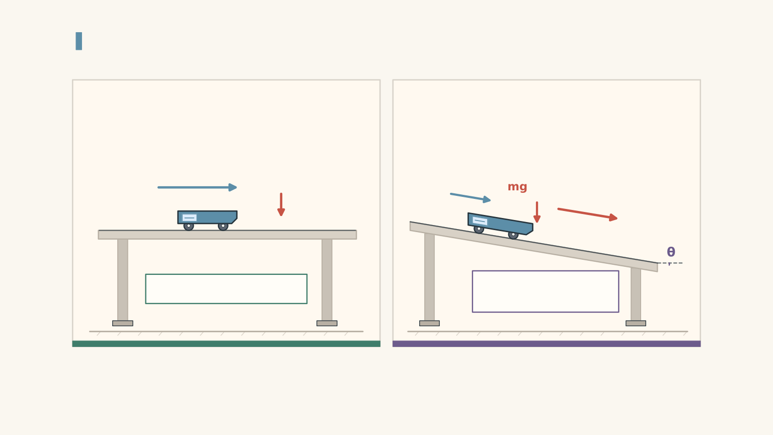
Connected masses share one acceleration magnitude
| Trolley on horizontal track | m_t Accelerates to the right along the track. Contributes to the total moving mass. |
|---|---|
| Hanging mass | m_h Accelerates downward as it drives the system. Shares the trolley’s acceleration magnitude for a taut, light string. |
01Understand what you are testing
Newton’s second law states that the net force acting on an object equals its mass multiplied by its acceleration:
\[ F_{\text{net}}=ma \]
Here:
- \(F_{\text{net}}\) is the net force, measured in newtons (N).
- \(m\) is the mass of the object or system being accelerated, measured in kilograms (kg).
- \(a\) is the acceleration, measured in metres per second squared (\(\mathrm{m\,s^{-2}}\)).
Rearranging the equation gives:
\[ a=\frac{F_{\text{net}}}{m} \]
This form makes the experimental predictions easier to see. Acceleration increases when net force increases, provided mass stays constant. Acceleration decreases when mass increases, provided net force stays constant.
But there’s an important word in the equation: net.
Why the net force matters
Imagine two people tugging a backpack in opposite directions. One pulls right with a force of 10 N, while the other pulls left with a force of 4 N. The net force is 6 N to the right, not 14 N.
The analogy has one job: to show that opposing forces must be accounted for. In an experiment, you must also identify the system you’re studying and the direction in which each force acts.
For a trolley pulled by a hanging mass, the hanging mass’s weight provides the driving force. Rolling resistance and pulley resistance oppose the motion.
If \(m_h\) is the hanging mass, \(g\) is gravitational field strength, and \(F_r\) is the total resisting force, the driving force is \(m_hg\). The net force along the system’s direction of motion is therefore
\[ F_{\text{net}}=m_hg-F_r \]
The acceleration becomes
\[ a=\frac{m_hg-F_r}{M} \]
Here, \(M\) is the total moving mass: the trolley, its added loads, the hanger, and any other moving components included in the model. The string’s mass is normally treated as negligible.
For a typical school experiment, use \(g=9.8\,\mathrm{m\,s^{-2}}\).
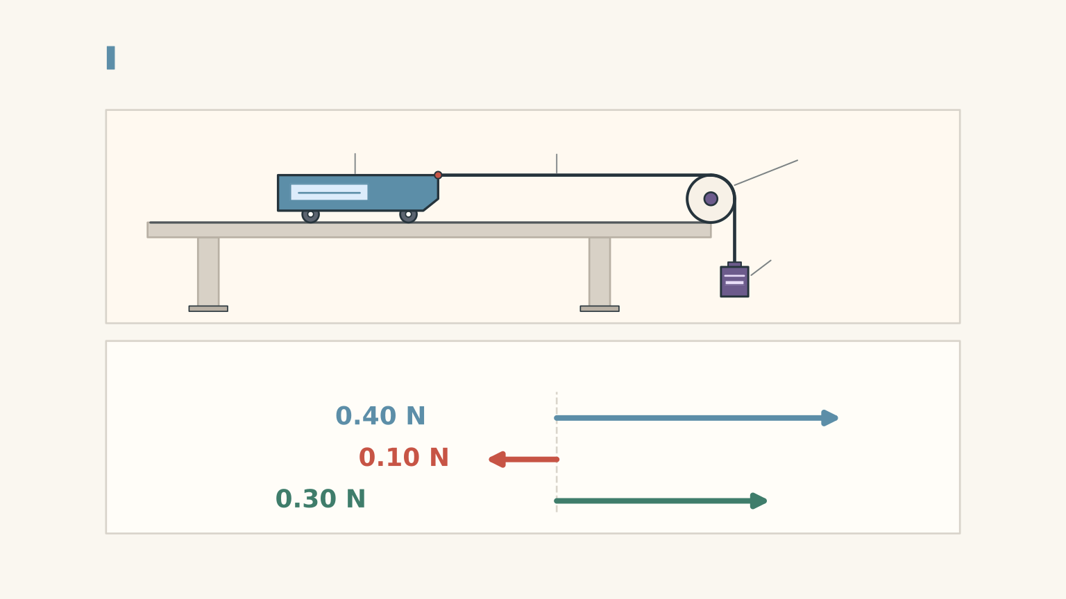
The distinction is easy to miss. A hanging mass of \(0.050\,\mathrm{kg}\) has a weight of \(0.490\,\mathrm{N}\), but if resistance is \(0.090\,\mathrm{N}\), the net force is only \(0.400\,\mathrm{N}\).
Using the hanging weight as though it were automatically the net force will overestimate the predicted acceleration.
02Set up a reliable experiment
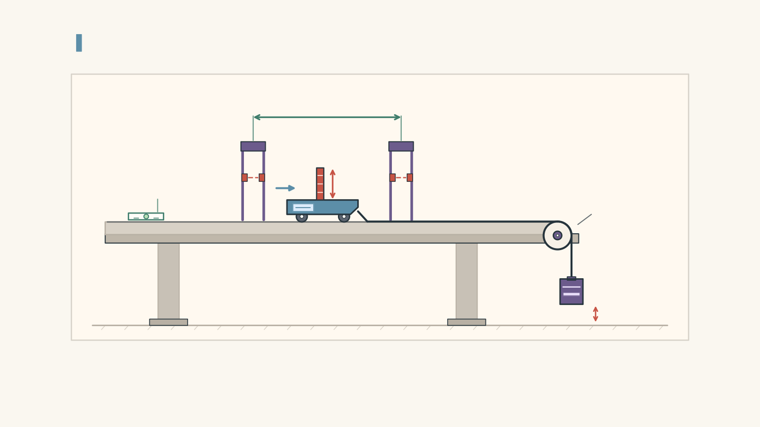
A standard school-laboratory setup uses:
- A trolley and a horizontal track.
- A pulley, light string, and mass hanger.
- Slotted masses that can be transferred between the trolley and hanger.
- A digital balance to measure mass.
- A motion sensor or two light gates to measure acceleration.
- A force sensor, if available, to measure applied forces and help account for resistance.
Before collecting data, check three things.
Level the track. A slight incline introduces a component of gravitational force along the track. This can assist or oppose the motion and create a systematic error.
Measure the complete moving mass. Don’t record only the trolley’s mass. Include the hanger and attached loads if they accelerate with the trolley.
Use a consistent release. Start from the same position, keep the string taut, and release the trolley without pushing it. Make sure the hanger cannot hit the floor before the measurement finishes and the trolley cannot collide with the pulley.
Measuring acceleration
A motion sensor can produce a velocity-time graph. The gradient of this graph gives the acceleration:
\[ a=\frac{\Delta v}{\Delta t} \]
where \(\Delta v\) is the change in velocity and \(\Delta t\) is the corresponding time interval.
Use a best-fit line rather than calculating a gradient from two arbitrarily chosen points. This helps reduce the effect of noisy measurements.
If your school uses two light gates, you can calculate the speed at each gate from the flag’s length and the time for which it blocks the beam. If the trolley’s speeds are \(v_1\) and \(v_2\), and the gates are separated by a distance \(\Delta x\), then
\[ a=\frac{v_2^2-v_1^2}{2\Delta x} \]
This follows from the constant-acceleration equation \(v^2=u^2+2as\).
Whichever method you use, measure acceleration rather than assuming that a heavier pull or a heavier trolley must produce a particular result.
03Experiment A: vary force while keeping mass constant
The first investigation tests whether acceleration is directly proportional to net force.
Variables
- Independent variable: net force, \(F_{\text{net}}\).
- Dependent variable: acceleration, \(a\).
- Controlled variable: total moving mass, \(M\).
Also keep the track angle, release method, measurement arrangement, and trolley as consistent as possible.
Method
Step 1: Measure the total moving mass of the system.
Step 2: Choose several different force settings. Aim for at least five settings across a useful range.
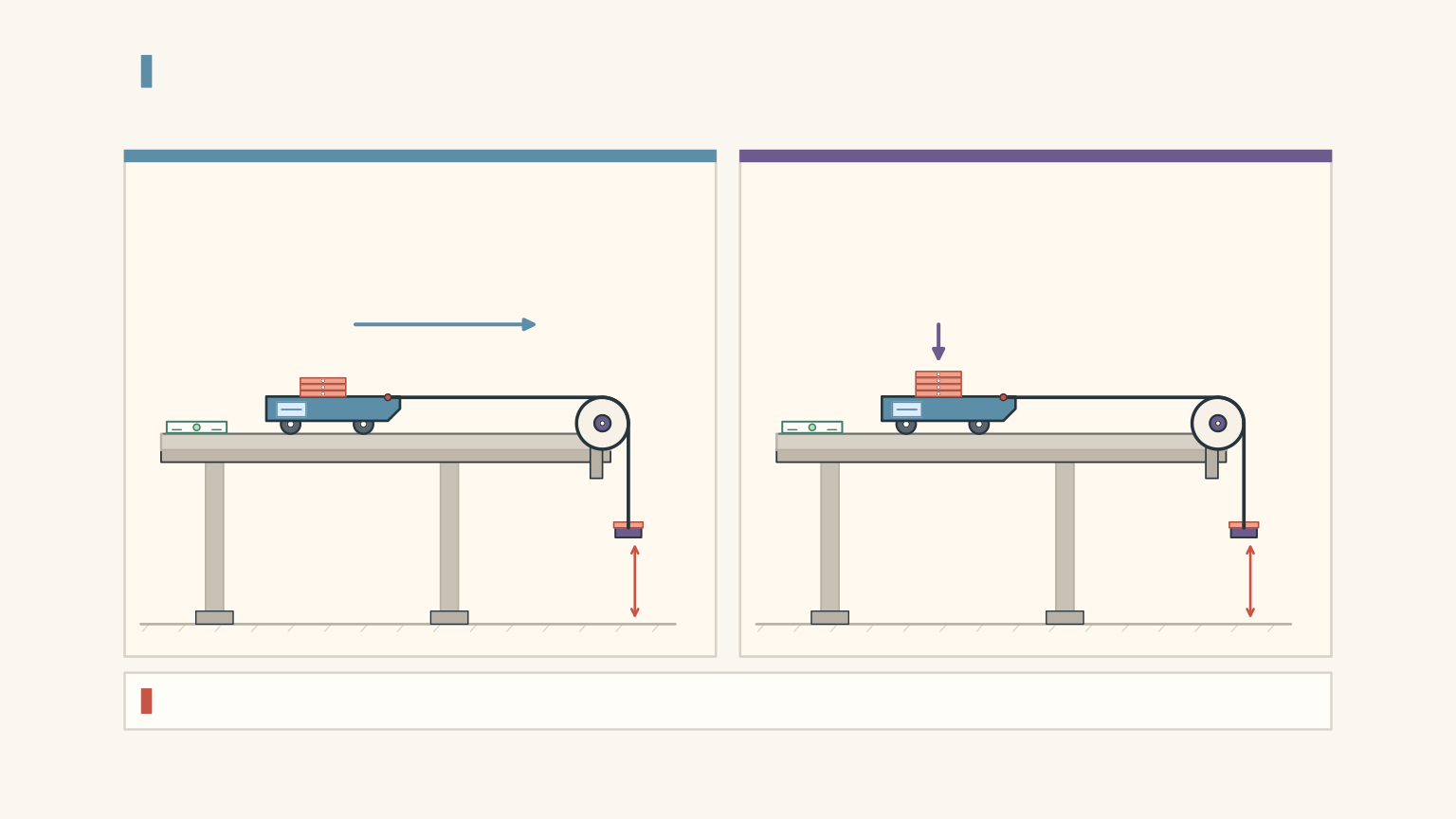
Step 3: If you’re using a trolley and hanger, transfer small slotted masses from the trolley to the hanger. This increases the hanging weight while keeping the total moving mass approximately constant.
Step 4: For each setting, measure the acceleration. Record the hanging mass, total moving mass, and any estimate of the resisting force.
Step 5: Calculate the net force for each run. If you use a horizontal force sensor instead, calculate the net force by subtracting the opposing resistance from the measured pull.
Step 6: Repeat each setting three to five times, then calculate the mean acceleration.
One complication deserves attention. Transferring mass from the trolley to the hanger changes the load pressing on the track. Rolling resistance may therefore change slightly. A force sensor and a suitable resistance measurement can improve the test. If you use a basic low-friction trolley, state that resistance is being treated as negligible or approximately constant rather than pretending it is exactly zero.
Worked example: correct for resistance
A trolley-hanger system has a total moving mass of \(1.20\,\mathrm{kg}\). The hanging mass is \(0.060\,\mathrm{kg}\), and the total resisting force is \(0.12\,\mathrm{N}\). Calculate the predicted acceleration. Take \(g=9.8\,\mathrm{m\,s^{-2}}\).
Step 1
\[ \begin{aligned} F_{\text{drive}}&=m_hg\\ &=0.060\times9.8\\ &=0.588\,\mathrm{N} \end{aligned} \]
Step 2
\[ \begin{aligned} F_{\text{net}}&=F_{\text{drive}}-F_r\\ &=0.588-0.12\\ &=0.468\,\mathrm{N} \end{aligned} \]
Step 3
\[ \begin{aligned} a&=\frac{F_{\text{net}}}{M}\\ &=\frac{0.468}{1.20}\\ &=0.390\,\mathrm{m\,s^{-2}} \end{aligned} \]
The predicted acceleration is \(0.390\,\mathrm{m\,s^{-2}}\).
If you ignored resistance, you would predict \(0.588/1.20=0.490\,\mathrm{m\,s^{-2}}\). That is a substantial difference, even though the resisting force is much smaller than the driving force.
The lesson is practical: a small unaccounted force can shift every data point, not just one result.
04Experiment B: vary mass while keeping net force constant
The second investigation tests whether acceleration is inversely proportional to mass.
Variables
- Independent variable: total moving mass, \(M\).
- Dependent variable: acceleration, \(a\).
- Controlled variable: net force, \(F_{\text{net}}\).
Keep the track angle, release method, force direction, and measurement setup consistent as well.
Method
Step 1: Choose a target net force.
Step 2: Set the total moving mass to a starting value and measure its acceleration.
Step 3: Add known masses to the trolley, measuring the complete moving mass each time.
Step 4: Maintain the same net force for each load and measure the acceleration.
Step 5: Repeat each setting three to five times and calculate the mean acceleration.
There’s a trap in the standard trolley-hanger version of this experiment. Keeping the hanging mass fixed keeps its weight constant, but it does not necessarily keep the net force constant. Adding mass to the trolley can increase rolling resistance.
For a more rigorous test, use a calibrated horizontal puller or force sensor. Measure the resistance for each load and adjust the applied pull so that the difference between the pull and the resistance remains constant.
If you only have a trolley, hanger, and light gates, you can still perform the standard approximate experiment. Just acknowledge the limitation and avoid claiming that the net force was held exactly constant unless you have checked it.
What should happen?
From Newton’s second law,
\[ a=\frac{F_{\text{net}}}{M} \]
If \(F_{\text{net}}\) stays constant, doubling \(M\) halves \(a\). Tripling \(M\) reduces \(a\) to one-third of its original value.
Notice that this is an inverse relationship, not a direct one. You should not expect a graph of acceleration against mass to be a straight line.
05Choose the right graph
Graphs are not just a way to display results. A well-chosen graph lets you test the mathematical relationship and estimate a physical quantity from its gradient.
Graph A: acceleration against net force
For the constant-mass experiment,
\[ a=\frac{1}{M}F_{\text{net}} \]
This has the form \(y=mx\), where the graph’s gradient is \(1/M\).
Plot:
- Horizontal axis: net force, \(F_{\text{net}}\), in N.
- Vertical axis: acceleration, \(a\), in \(\mathrm{m\,s^{-2}}\).
If Newton’s second law is supported by the data, the points should lie approximately along a straight line. If resistance has been properly accounted for, the line should pass near the origin.
The gradient has units of \(\mathrm{kg^{-1}}\), so the experimental mass can be calculated from
\[ M=\frac{1}{\text{gradient}} \]
You can also plot net force against acceleration. In that case, the gradient is the mass itself, in kilograms.
Graph B: acceleration against reciprocal mass
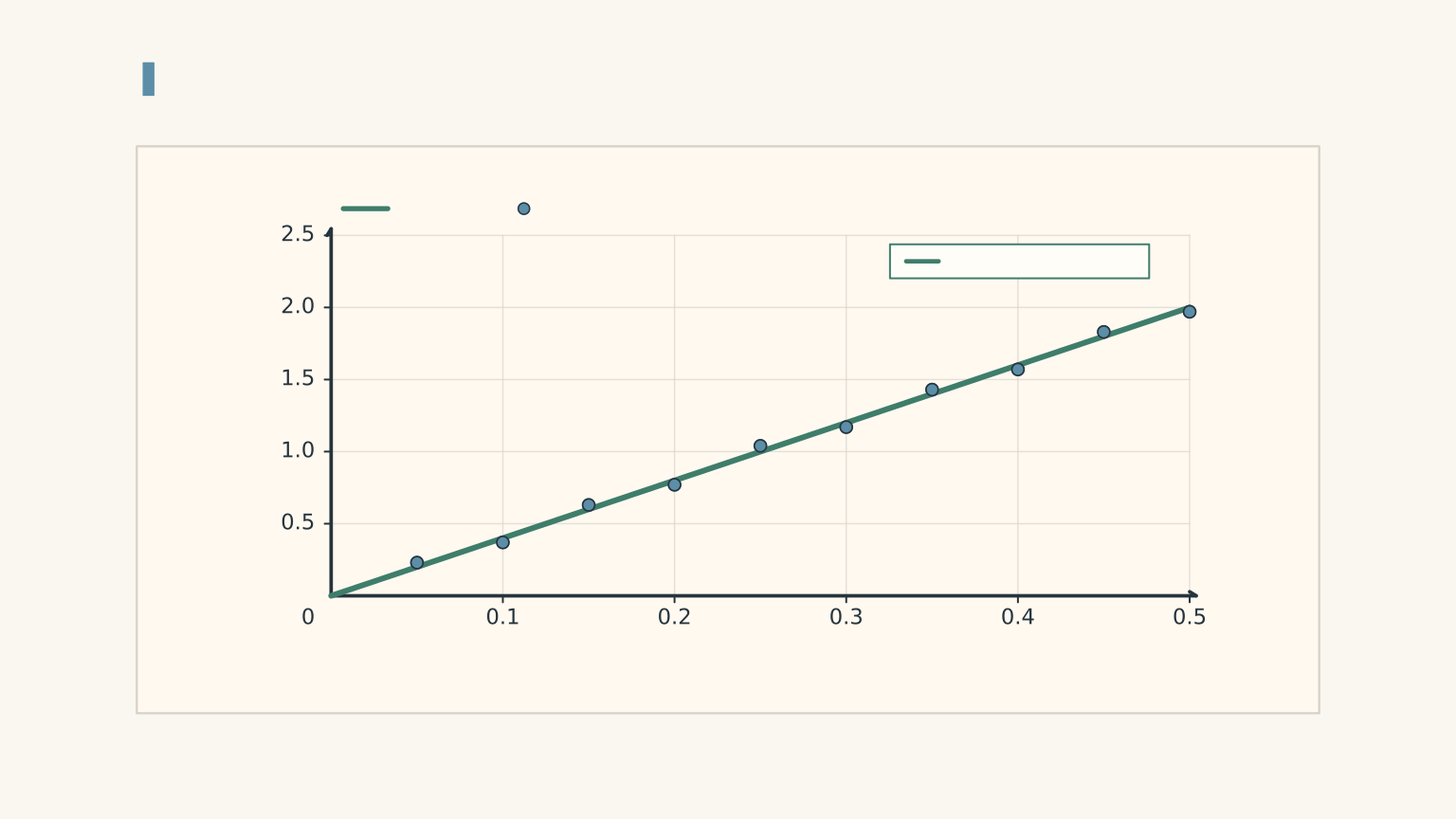
For the constant-net-force experiment,
\[ a=F_{\text{net}}\left(\frac{1}{M}\right) \]
Plot:
- Horizontal axis: reciprocal mass, \(1/M\), in \(\mathrm{kg^{-1}}\).
- Vertical axis: acceleration, \(a\), in \(\mathrm{m\,s^{-2}}\).
The gradient is now \(F_{\text{net}}\), measured in newtons.
A straight-line relationship supports the prediction that acceleration is proportional to reciprocal mass when net force is constant.
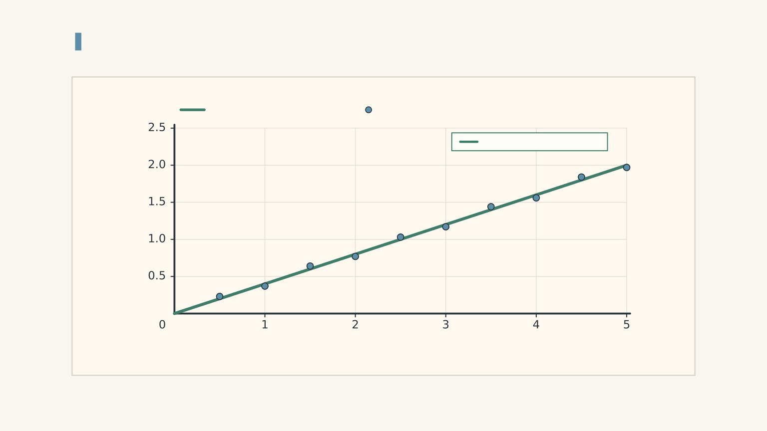
Why not simply plot acceleration against mass? Because \(a=F_{\text{net}}/M\) is an inverse relationship. The resulting graph curves rather than forming a straight line.
Worked example: use a graph to estimate mass
A student keeps the total moving mass fixed and obtains the following results.
| Net force (N) | Acceleration (\(\mathrm{m\,s^{-2}}\)) |
|---|---|
| 0.10 | 0.13 |
| 0.20 | 0.25 |
| 0.30 | 0.38 |
| 0.40 | 0.50 |
A balance gives a total moving mass of \(0.80\,\mathrm{kg}\). Use the first and last data points to estimate the gradient of the acceleration-versus-net-force graph, calculate the experimental mass, and compare it with the measured mass.
Step 1
\[ \begin{aligned} \text{gradient} &=\frac{\Delta a}{\Delta F_{\text{net}}}\\ &=\frac{0.50-0.13}{0.40-0.10}\\ &=\frac{0.37}{0.30}\\ &=1.23\,\mathrm{kg^{-1}} \end{aligned} \]
The units are inverse kilograms because dividing acceleration by force gives \((\mathrm{m\,s^{-2}})/\mathrm{N}=\mathrm{kg^{-1}}\).
Step 2
\[ \begin{aligned} M_{\text{experimental}} &=\frac{1}{1.23}\\ &\approx0.81\,\mathrm{kg} \end{aligned} \]
Step 3
The experimental value is approximately \(0.81\,\mathrm{kg}\), compared with the balance reading of \(0.80\,\mathrm{kg}\). The difference is about \(0.01\,\mathrm{kg}\), or roughly 1.4%.
The results are consistent with the expected relationship to a close approximation. The small difference could arise from measurement uncertainty, resistance corrections, or the use of rounded data. It is not sensible to demand that experimental measurements reproduce the theoretical value exactly.
06Make your results believable
A straight-looking graph is useful, but it is not the whole investigation. Your conclusion depends on how well you controlled the variables and how reliably you measured acceleration.
Repeat trials and calculate a mean
At each force or mass setting, perform three to five trials where practical.
Suppose three acceleration readings are \(0.31\), \(0.34\), and \(0.32\,\mathrm{m\,s^{-2}}\). The mean is
\[ \bar a=\frac{0.31+0.34+0.32}{3} =0.323\,\mathrm{m\,s^{-2}} \]
The mean reduces the influence of random variation, but it does not eliminate systematic errors. If the track is tilted, repeating the same flawed setup will not fix it.
Record all reasonable trials. If a run includes a clear collision or a sensor failure, document what happened and repeat it rather than quietly removing a result that doesn’t fit your prediction.
Recognise the main sources of error
| Source of error | How it affects the investigation | What to do |
|---|---|---|
| Rolling resistance | Reduces the net force compared with the driving force. | Measure or estimate resistance, or state that it is treated as negligible. |
| Pulley resistance | Makes the actual driving force less effective than the ideal model predicts. | Use a smooth pulley and account for resistance where possible. |
| Track not level | Adds a force component along the track. | Check and level the track before testing. |
| Inconsistent release | An accidental push changes the initial motion. | Release the trolley without pushing it. |
| Sensor resolution | Makes small changes in acceleration difficult to distinguish. | Use an appropriate measurement range and repeat trials. |
| Incorrect mass | Produces an incorrect prediction or graph gradient. | Include every moving component in the mass calculation. |
The direction of the error matters. If the force is overestimated because resistance was ignored, the predicted acceleration will be too high. If the track slopes down in the direction of motion, gravity may increase the measured acceleration.
Interpret the graph instead of forcing it to agree
A non-zero intercept is not automatically evidence against Newton’s second law.
If you plot acceleration against the hanger’s driving force without subtracting an approximately constant resistance, the relationship becomes
\[ a=\frac{F_{\text{drive}}-F_r}{M} \]
The graph can still be linear, but it will have a negative vertical intercept of \(-F_r/M\). Subtracting the resistance before plotting should move the intercept closer to zero.
A curved graph might indicate that resistance changes with the load, that the force was not held constant, or that the system behaved differently at different speeds. Check these possibilities before concluding that the relationship failed.
Your final conclusion should say what the results support, identify the main limitations, and distinguish experimental evidence from the ideal model. For example, you might conclude that acceleration was approximately proportional to net force at constant mass, with a small discrepancy attributable to resistance and measurement uncertainty.
07Questions and solutions
Question 1
A trolley with a total moving mass of \(0.75\,\mathrm{kg}\) experiences a net force of \(1.5\,\mathrm{N}\). Calculate its acceleration.
Solution 1
The acceleration is \(2.0\,\mathrm{m\,s^{-2}}\). Newton’s second law gives
\[ \begin{aligned} a&=\frac{F_{\text{net}}}{M}\\ &=\frac{1.5}{0.75}\\ &=2.0\,\mathrm{m\,s^{-2}} \end{aligned} \]
The units are correct because a newton is equivalent to \(\mathrm{kg\,m\,s^{-2}}\). The result means that the trolley’s velocity changes by \(2.0\,\mathrm{m\,s^{-1}}\) every second while this net force remains constant.
Question 2
A trolley-hanger system has a total moving mass of \(1.40\,\mathrm{kg}\). The hanger has a mass of \(0.040\,\mathrm{kg}\), and the total resisting force is \(0.080\,\mathrm{N}\). Take \(g=9.8\,\mathrm{m\,s^{-2}}\).
Calculate the corrected acceleration. A student ignores resistance and calculates the acceleration using the hanging weight alone. By what percentage does the student’s estimate exceed the corrected value?
Solution 2
The corrected acceleration is approximately \(0.223\,\mathrm{m\,s^{-2}}\), and the student’s friction-free estimate is about 25.6% higher than this value.
First, calculate the hanging weight:
\[ \begin{aligned} F_{\text{drive}}&=m_hg\\ &=0.040\times9.8\\ &=0.392\,\mathrm{N} \end{aligned} \]
Subtract the resisting force:
\[ F_{\text{net}}=0.392-0.080=0.312\,\mathrm{N} \]
Then calculate the corrected acceleration:
\[ \begin{aligned} a&=\frac{0.312}{1.40}\\ &=0.2229\,\mathrm{m\,s^{-2}} \end{aligned} \]
If resistance is ignored, the student’s estimate is
\[ a_{\text{student}}=\frac{0.392}{1.40} =0.280\,\mathrm{m\,s^{-2}} \]
The percentage by which this exceeds the corrected result is
\[ \begin{aligned} \%\text{ excess} &=\frac{0.280-0.2229}{0.2229}\times100\\ &\approx25.6\% \end{aligned} \]
The student’s calculation is mathematically correct for an ideal system with no resistance. The error is using the driving force as though it were the net force in a real experiment.
Question 3
A student keeps the total moving mass fixed and records these results.
| Net force (N) | Acceleration (\(\mathrm{m\,s^{-2}}\)) |
|---|---|
| 0.10 | 0.13 |
| 0.20 | 0.25 |
| 0.30 | 0.38 |
| 0.40 | 0.50 |
Use the first and last points to estimate the gradient of an acceleration-versus-net-force graph. Calculate the experimental mass and compare it with a balance reading of \(0.80\,\mathrm{kg}\). Does the data support a direct relationship between acceleration and net force?
Solution 3
The experimental mass is approximately \(0.81\,\mathrm{kg}\), and the data support an approximately direct relationship between acceleration and net force.
The gradient is
\[ \begin{aligned} \text{gradient} &=\frac{0.50-0.13}{0.40-0.10}\\ &=\frac{0.37}{0.30}\\ &=1.23\,\mathrm{kg^{-1}} \end{aligned} \]
For constant mass, the model predicts
\[ a=\frac{1}{M}F_{\text{net}} \]
Therefore, the gradient is the reciprocal of the mass:
\[ M=\frac{1}{1.23}\approx0.81\,\mathrm{kg} \]
This is close to the balance reading of \(0.80\,\mathrm{kg}\). The acceleration also increases approximately linearly as net force increases.
The data support the model, but they do not establish exact proportionality beyond all doubt. Measurement uncertainty and a small systematic offset may explain the differences between the points and an ideal line through the origin.
Question 4
A student uses a force sensor to maintain a measured net force of \(0.60\,\mathrm{N}\) while varying the total moving mass. The mass uncertainty is negligible, and each acceleration measurement has an uncertainty of \(\pm0.03\,\mathrm{m\,s^{-2}}\).
| Total moving mass (kg) | Measured acceleration (\(\mathrm{m\,s^{-2}}\)) |
|---|---|
| 0.50 | \(1.12\pm0.03\) |
| 0.75 | \(0.79\pm0.03\) |
| 1.00 | \(0.61\pm0.03\) |
A student plots acceleration against mass and argues that the inverse relationship has failed because the points do not form a straight line.
Identify the appropriate graph, calculate \(Ma\) for each run, and determine which result should be checked first. Explain why the data do not automatically disprove Newton’s second law.
Solution 4
The appropriate graph is acceleration against reciprocal mass, \(1/M\), and the first run should be checked first because its result is inconsistent with the stated uncertainty.
For a constant net force,
\[ a=F_{\text{net}}\left(\frac{1}{M}\right) \]
This predicts a straight line when \(a\) is plotted against \(1/M\), not when \(a\) is plotted against \(M\).
Now calculate the product \(Ma\) for each run:
| Mass (kg) | Acceleration (\(\mathrm{m\,s^{-2}}\)) | \(Ma\) (N) |
|---|---|---|
| 0.50 | 1.12 | 0.560 |
| 0.75 | 0.79 | 0.5925 |
| 1.00 | 0.61 | 0.610 |
If the net force is \(0.60\,\mathrm{N}\), the predicted accelerations are
\[ \begin{aligned} a_{0.50}&=\frac{0.60}{0.50}=1.20\,\mathrm{m\,s^{-2}}\\ a_{0.75}&=\frac{0.60}{0.75}=0.80\,\mathrm{m\,s^{-2}}\\ a_{1.00}&=\frac{0.60}{1.00}=0.60\,\mathrm{m\,s^{-2}} \end{aligned} \]
The second and third readings are consistent with these predictions within the stated uncertainty. The first reading differs by \(0.08\,\mathrm{m\,s^{-2}}\), which exceeds its uncertainty of \(0.03\,\mathrm{m\,s^{-2}}\).
Repeat the first run and check the recorded mass, force trace, and acceleration measurement. Don’t simply discard the point.
The original argument fails for two reasons. First, acceleration against mass is not expected to be linear. Second, one inconsistent measurement does not establish that the physical model is wrong. The correct graph and a check of the measurement uncertainty are needed before drawing that conclusion.
Question 5
Two students investigate a trolley-hanger system. All masses listed below are total moving masses, including every component that accelerates.
In Set A, the total moving mass stays at \(1.00\,\mathrm{kg}\). The hanging weight and measured acceleration are:
| Hanging weight (N) | Measured acceleration (\(\mathrm{m\,s^{-2}}\)) |
|---|---|
| 0.20 | 0.10 |
| 0.30 | 0.20 |
| 0.40 | 0.30 |
The resisting force is measured as \(0.10\,\mathrm{N}\) in every run.
In Set B, the hanging weight stays at \(0.30\,\mathrm{N}\), but the total moving mass changes.
| Total moving mass (kg) | Resisting force (N) | Measured acceleration (\(\mathrm{m\,s^{-2}}\)) |
|---|---|---|
| 1.00 | 0.10 | 0.20 |
| 1.50 | 0.12 | 0.12 |
| 2.00 | 0.14 | 0.08 |
Student A claims that Set A disproves \(F_{\text{net}}=Ma\), because the hanging weight divided by the total mass does not equal the measured acceleration in the first run.
Student B claims that Set B proves \(a\propto1/M\), because acceleration decreases as mass increases.
Evaluate both claims. Then design a fairer mass experiment using a calibrated horizontal puller. For total moving masses of \(1.00\), \(1.50\), and \(2.00\,\mathrm{kg}\), the measured resistive forces are \(0.10\), \(0.12\), and \(0.14\,\mathrm{N}\), respectively. If the target net force is \(0.20\,\mathrm{N}\), calculate the pull required for each mass and predict the resulting accelerations.
Solution 5
Neither student has interpreted the experiment correctly. Set A is consistent with Newton’s second law after resistance is subtracted. Set B is also consistent with the law in each individual run, but it does not establish the inverse-mass relationship because the net force changes between runs.
Set A: subtract resistance first.
For each run,
\[ F_{\text{net}}=F_{\text{hanging}}-F_r \]
The net forces are \(0.10\), \(0.20\), and \(0.30\,\mathrm{N}\).
Since the total mass is \(1.00\,\mathrm{kg}\), the predicted accelerations are
\[ a=\frac{F_{\text{net}}}{M} \]
giving \(0.10\), \(0.20\), and \(0.30\,\mathrm{m\,s^{-2}}\), respectively.
These agree with the measured accelerations. Student A has used the hanging weight instead of the net force, so the apparent contradiction disappears once resistance is included.
Set B: check whether the net force stays constant.
The hanging weight remains \(0.30\,\mathrm{N}\), but the resisting force increases with mass.
| Mass (kg) | Net force (N) | \(Ma\) (N) |
|---|---|---|
| 1.00 | \(0.30-0.10=0.20\) | \(1.00\times0.20=0.20\) |
| 1.50 | \(0.30-0.12=0.18\) | \(1.50\times0.12=0.18\) |
| 2.00 | \(0.30-0.14=0.16\) | \(2.00\times0.08=0.16\) |
Each run satisfies \(F_{\text{net}}=Ma\). However, the net force decreases from \(0.20\) to \(0.16\,\mathrm{N}\) as the mass increases.
Student B is right that acceleration decreases, but that observation alone does not establish \(a\propto1/M\). To test that specific relationship, net force must stay constant.
Redesign the mass experiment.
The horizontal puller must overcome resistance while maintaining a net force of \(0.20\,\mathrm{N}\). Therefore,
\[ F_{\text{pull}}=F_{\text{net}}+F_r \]
For the three masses, the required pulls are:
\[ \begin{aligned} F_{\text{pull},1}&=0.20+0.10=0.30\,\mathrm{N}\\ F_{\text{pull},2}&=0.20+0.12=0.32\,\mathrm{N}\\ F_{\text{pull},3}&=0.20+0.14=0.34\,\mathrm{N} \end{aligned} \]
Now the net force is \(0.20\,\mathrm{N}\) in every run. The predicted accelerations are
\[ \begin{aligned} a_1&=\frac{0.20}{1.00}=0.20\,\mathrm{m\,s^{-2}}\\ a_2&=\frac{0.20}{1.50}\approx0.133\,\mathrm{m\,s^{-2}}\\ a_3&=\frac{0.20}{2.00}=0.10\,\mathrm{m\,s^{-2}} \end{aligned} \]
Plot these measured accelerations against reciprocal mass. If the experiment supports the model, the points should lie approximately along a straight line with a gradient of \(0.20\,\mathrm{N}\).
The crucial distinction is that a changing mass and a changing net force can produce a trend that looks reasonable without isolating the relationship you intended to test. A fair experiment controls the actual physical quantity in the equation, not merely a convenient substitute for it.
Once your force and mass tests are complete, the next useful step is uncertainty analysis: compare your measured graph gradients and intercepts with their predicted values, and decide whether any differences are significant relative to the limitations of your measurements.