
Mean, Range and Standard Deviation for HSC Science Practicals
Learn how to calculate and interpret the mean, range, sample standard deviation, and standard uncertainty in repeated experimental measurements. Includes worked Physics and Chemistry examples explaining precision, accuracy, and percentage error.
Five measurements of a pendulum’s period are 1.42 s, 1.39 s, 1.41 s, 1.43 s, and 1.40 s. Their average is 1.41 s. But is that enough information to report a reliable experimental result?
The readings differ by as much as 0.04 s. Does that mean the period is uncertain by 0.04 s? Or does averaging several measurements give us a more precise estimate?
These are different questions, and answering them requires four ideas: the mean, the range, the standard deviation, and the standard uncertainty in the mean. Understanding the difference is essential when analysing Physics and Chemistry practical results.
01Why do we repeat measurements?
Imagine measuring the period of a simple pendulum. You release a bob from a small angle and use a stopwatch to time its oscillations.
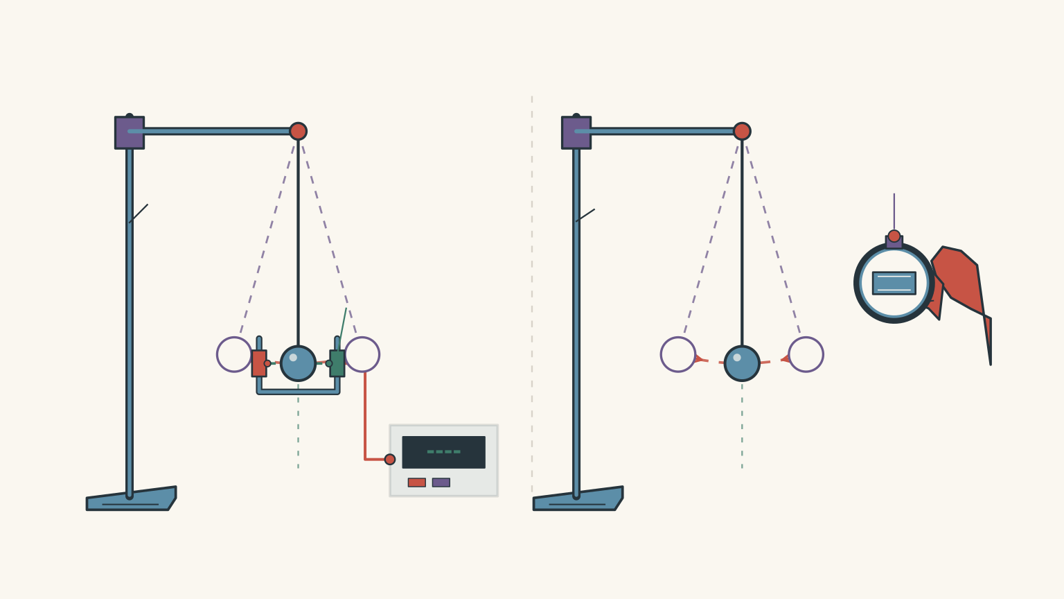
The apparatus is straightforward. A clamp stand supports a pivot, a string hangs from the pivot, and a bob is attached to the bottom. A ruler beside the string allows you to measure its length.
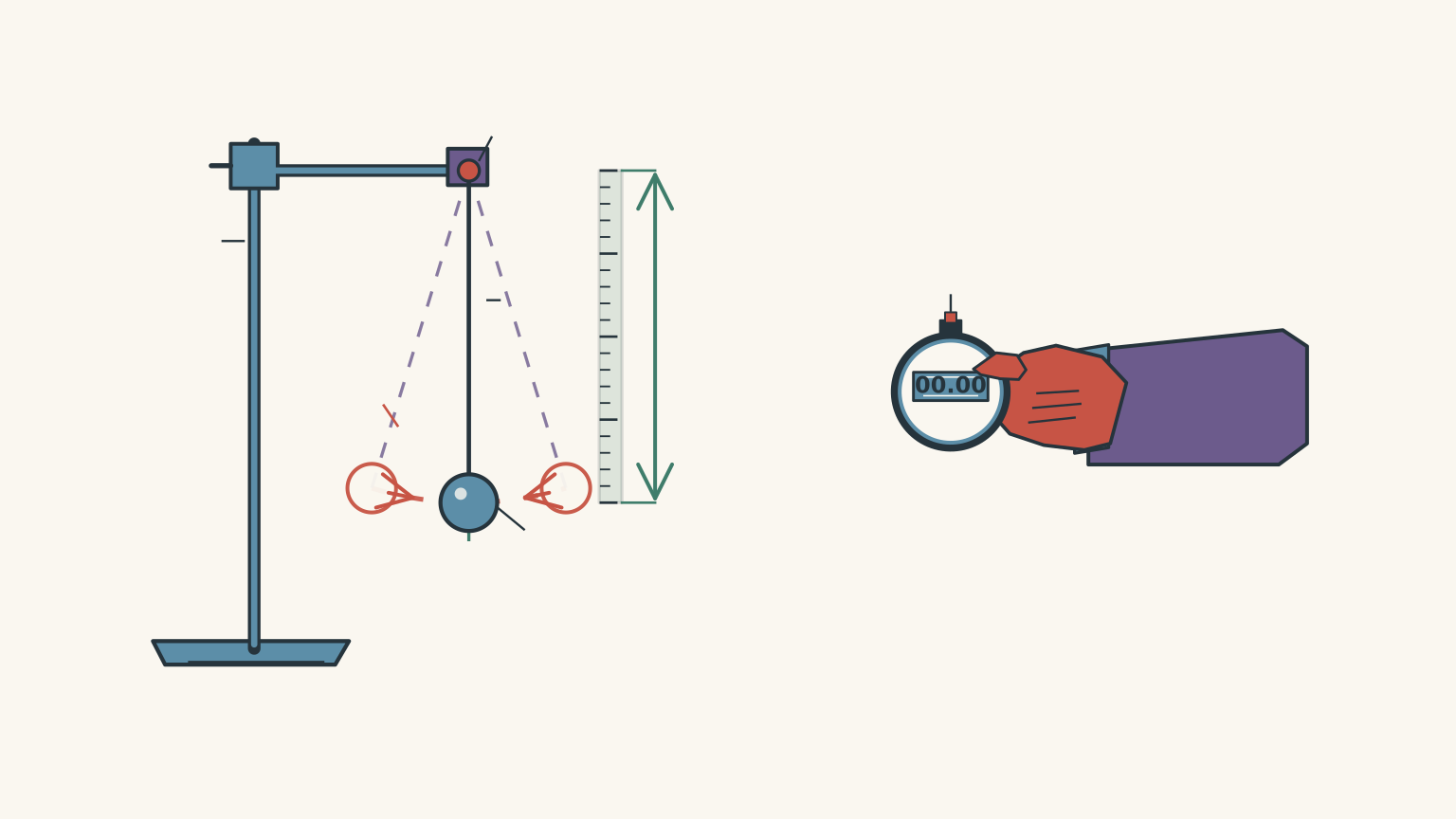
Suppose you time one complete oscillation five times.
You might expect to obtain exactly the same result each time. In reality, your measurements will probably differ slightly because of:
- Human reaction time when starting and stopping the stopwatch.
- The limited resolution of the stopwatch.
- Small differences in how you identify the start and end of an oscillation.
- Minor changes in the release conditions.
These variations are called random errors. They cause repeated measurements to scatter around an underlying value.
Your first experimental design might be to time just one oscillation. However, human reaction time can be a significant fraction of such a short measurement.
A better approach is to time ten complete oscillations and divide the total time by ten.
For example, if ten oscillations take 14.1 s:
\[ T=\frac{14.1}{10}=1.41\text{ s} \]
Here, \(T\) is the period, or time taken for one complete oscillation.
If the combined start-and-stop timing variation is approximately 0.2 s, dividing the total time by ten reduces its contribution to the calculated period to approximately 0.02 s.
The timing variation has not disappeared. However, its effect on each calculated period is smaller.
This revised method gives us a more useful set of measurements to analyse.
The central prediction is that, provided the pendulum’s length and release conditions remain constant, the period should remain approximately constant. Our measurements should therefore cluster around a common value.
The statistical methods below help us describe that cluster.
01The mean: finding the central value
The mean is the arithmetic average of a set of measurements.
It gives us a single value that represents the centre of our experimental results.
To calculate it, add all the measurements and divide by the number of measurements.
\[ \bar{x}=\frac{\sum x_i}{n} \]
Where:
- \(\bar{x}\) is the sample mean.
- \(x_i\) represents an individual measurement.
- \(n\) is the total number of measurements.
- \(\sum\) means to add all the measurements together.
For example, consider five measurements:
\[ 1.42,\quad 1.39,\quad 1.41,\quad 1.43,\quad 1.40 \]
The mean is:
\[ \begin{aligned} \bar{x} &=\frac{1.42+1.39+1.41+1.43+1.40}{5}\\ &=\frac{7.05}{5}\\ &=1.41\text{ s} \end{aligned} \]
The mean period is therefore 1.41 s.
Notice that 1.41 s does not have to be one of the measurements, although it happens to be in this example.
The mean gives us a central estimate, but it does not tell us how closely grouped the measurements are.
For that, we need to look at the spread.
02The range: measuring the total spread
The range is the difference between the largest and smallest measurements.
\[ \text{Range}=x_{\max}-x_{\min} \]
Where:
- \(x_{\max}\) is the largest measurement.
- \(x_{\min}\) is the smallest measurement.
Using our pendulum data:
- Largest measurement = 1.43 s.
- Smallest measurement = 1.39 s.
Therefore:
\[ \text{Range}=1.43-1.39 \]
\[ \boxed{\text{Range}=0.04\text{ s}} \]
The measurements span a total interval of 0.04 s.
A smaller range generally suggests that repeated measurements are more closely grouped.
However, there is a limitation.
The range only considers the two extreme measurements. It ignores everything in between.
Consider these two sets:
| Set A (s) | Set B (s) |
|---|---|
| 1.40 | 1.40 |
| 1.40 | 1.41 |
| 1.41 | 1.42 |
| 1.41 | 1.43 |
| 1.44 | 1.44 |
Both sets have a range of 0.04 s.
However, their measurements are distributed differently.
This is why the range is a useful starting point, but not a complete description of experimental spread.
03Standard deviation: measuring how spread out the results are
Standard deviation gives us a more detailed measure of the spread of repeated measurements.
Rather than looking only at the highest and lowest values, it considers how far every measurement is from the mean.
Think of the mean as the centre of a group of measurements. Standard deviation tells us how tightly those measurements cluster around that centre.
A small standard deviation means the measurements are closely grouped.
A large standard deviation means they are more widely spread.
Calculating sample standard deviation
For repeated experimental measurements, we generally use the sample standard deviation:
\[ \boxed{ s=\sqrt{ \frac{\sum(x_i-\bar{x})^2}{n-1} } } \]
Where:
- \(s\) is the sample standard deviation.
- \(x_i\) is an individual measurement.
- \(\bar{x}\) is the mean.
- \(n\) is the number of measurements.
There are four steps hidden inside this equation.
Step 1: Calculate the mean.
We already know that the mean of our pendulum measurements is 1.41 s.
Step 2: Calculate each deviation from the mean.
Subtract the mean from each measurement.
For example:
\[ 1.42-1.41=0.01\text{ s} \]
Repeat this for every measurement.
Step 3: Square each deviation and add them together.
Squaring makes all contributions positive, so measurements above and below the mean do not cancel each other out.
Step 4: Divide by \(n-1\), then take the square root.
This gives the sample standard deviation in the original units of measurement.
Why do we divide by \(n-1\), not \(n\)?
This is an important distinction.
We are using a sample of measurements to estimate the spread of the underlying measurement process.
Because the mean is calculated from the same sample, the deviations from that mean are constrained: they must add to zero.
For five measurements, only four deviations can vary independently. The fifth is determined by the other four.
Dividing by \(n-1\) corrects for the tendency of a sample mean to underestimate the true population spread.
If we were calculating the standard deviation of an entire population rather than estimating it from a sample, we would divide by \(n\).
For ordinary HSC practical investigations involving repeated measurements, the sample standard deviation is generally the appropriate choice.
05Worked example: calculating the standard deviation of a pendulum
Five independent trials are conducted to measure the period of a pendulum. Each trial involves timing ten complete oscillations and dividing the total time by ten.
The calculated periods are:
\[ 1.42,\quad 1.39,\quad 1.41,\quad 1.43,\quad 1.40\text{ s} \]
Calculate the mean, range, sample standard deviation, and standard uncertainty in the mean.
Step 1Calculate the mean.
\[ \bar{x}=\frac{1.42+1.39+1.41+1.43+1.40}{5} \]
\[ \boxed{\bar{x}=1.41\text{ s}} \]
Step 2Calculate the range.
\[ \text{Range}=1.43-1.39 \]
\[ \boxed{\text{Range}=0.04\text{ s}} \]
Step 3Calculate the deviations from the mean.
| Measurement (s) | Deviation from mean (s) | Squared deviation (s²) |
|---|---|---|
| 1.42 | +0.01 | 0.0001 |
| 1.39 | -0.02 | 0.0004 |
| 1.41 | 0.00 | 0.0000 |
| 1.43 | +0.02 | 0.0004 |
| 1.40 | -0.01 | 0.0001 |
| Total | 0.00 | 0.0010 |
The sum of the squared deviations is:
\[ \sum(x_i-\bar{x})^2=0.0010\text{ s}^2 \]
Step 4Calculate the sample standard deviation.
There are five measurements, so \(n-1=4\).
\[ \begin{aligned} s&=\sqrt{\frac{0.0010}{5-1}}\\ &=\sqrt{0.00025}\\ &=0.01581\text{ s} \end{aligned} \]
Therefore:
\[ \boxed{s=0.016\text{ s}} \]
The standard deviation is approximately 0.016 s.
This describes the spread of the individual period measurements around their mean.
But there is another question worth asking: how precisely have we determined the mean itself?
04Standard uncertainty in the mean
This is where many students confuse two different quantities.
The standard deviation describes the spread of individual measurements.
The standard uncertainty in the mean describes how precisely we have estimated the mean from those measurements.
These are not interchangeable.
The standard uncertainty in the mean is calculated using:
\[ \boxed{ u_{\bar{x}}=\frac{s}{\sqrt{n}} } \]
Where:
- \(u_{\bar{x}}\) is the standard uncertainty in the mean.
- \(s\) is the sample standard deviation.
- \(n\) is the number of independent measurements.
Notice that the denominator is now \(\sqrt{n}\), not \(n-1\).
Why?
When we average several independent measurements, random variations tend to cancel out. As the number of measurements increases, the average generally becomes more precisely determined.
The uncertainty decreases in proportion to \(1/\sqrt{n}\).
For example:
- Four times as many independent measurements halves the standard uncertainty.
- Nine times as many independent measurements reduces it to one-third.
Importantly, this does not mean the individual measurements become less scattered. Their standard deviation may remain approximately the same.
Continuing the pendulum example
We calculated:
\[ s=0.01581\text{ s} \]
There were five measurements.
Therefore:
\[ \begin{aligned} u_{\bar{x}} &=\frac{0.01581}{\sqrt{5}}\\ &=0.00707\text{ s} \end{aligned} \]
So:
\[ \boxed{u_{\bar{x}}=0.007\text{ s}} \]
Our experimental result can therefore be reported as:
\[ \boxed{T=1.410\pm0.007\text{ s}} \]
The uncertainty here represents one standard uncertainty in the estimated mean, based on the observed random scatter.
It is not a guarantee that the true period lies within this interval. It also does not account for systematic errors, such as an incorrectly calibrated stopwatch.
Understanding the difference visually
A graph helps make these statistical quantities much easier to distinguish.
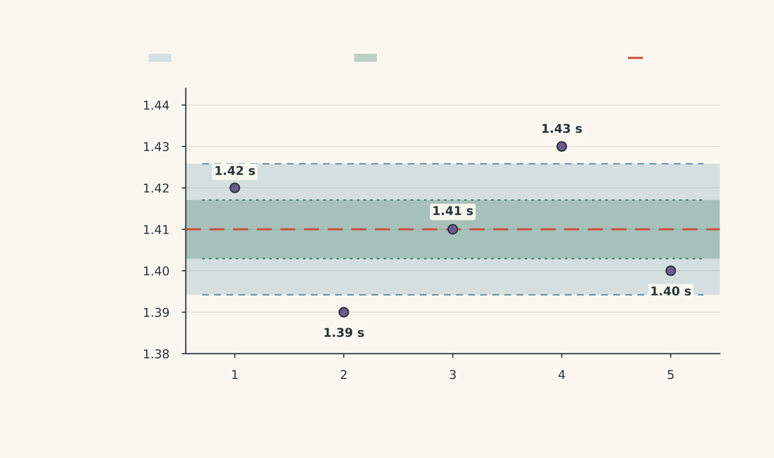
Notice three things:
- The horizontal line represents the mean period.
- The wider band represents one standard deviation either side of the mean. It describes the spread of individual readings.
- The narrower band represents one standard uncertainty either side of the mean. It describes the precision of the estimated average.
The individual measurements do not all need to fall inside the standard deviation band.
Also, the standard uncertainty band is not an interval that every individual measurement should fall inside. It relates to the estimated mean, not individual readings.
One more important observation: our measurements do not show a consistent upward or downward trend across the trials.
That supports treating them as repeated measurements of approximately the same quantity.
If they showed a clear trend, we would need to investigate before using the standard uncertainty formula.
05Applying the statistics to Chemistry practicals
The same statistical methods apply to Chemistry experiments.
Consider an acid-base titration.
A burette containing sodium hydroxide is clamped vertically above a conical flask containing a measured volume of hydrochloric acid and a suitable indicator.
You slowly release the sodium hydroxide through the burette tap while swirling the flask. When the endpoint is reached, you record the volume delivered.
You repeat the titration using fresh samples to obtain several titre measurements.
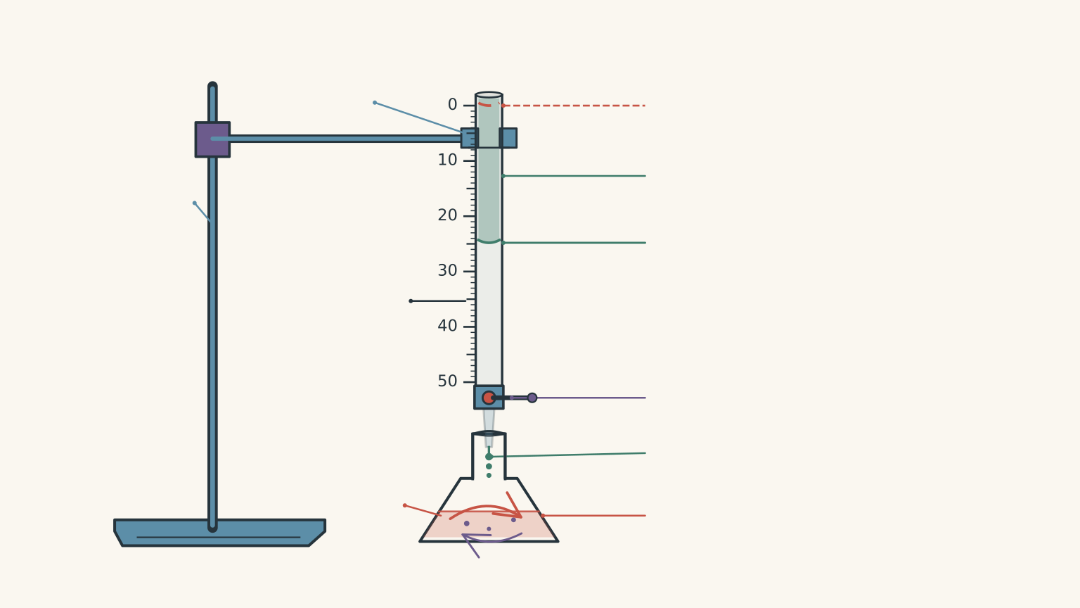
Suppose four concordant titres are obtained:
\[ 24.80,\quad24.75,\quad24.85,\quad24.80\text{ mL} \]
A reference value for the titre is known to be 25.00 mL.
Let’s analyse the results.
Worked example: analysing repeated titration results
Calculate the mean titre, range, sample standard deviation, standard uncertainty in the mean, percentage error, and percentage uncertainty in the mean.
Step 1Calculate the mean titre.
\[ \begin{aligned} \bar{x} &=\frac{24.80+24.75+24.85+24.80}{4}\\ &=\frac{99.20}{4}\\ &=24.80\text{ mL} \end{aligned} \]
Step 2Calculate the range.
\[ \text{Range}=24.85-24.75 \]
\[ \boxed{\text{Range}=0.10\text{ mL}} \]
Step 3Calculate the sample standard deviation.
The deviations from the mean are:
\[ 0,\quad-0.05,\quad+0.05,\quad0 \]
Their squared deviations add to:
\[ 0.0025+0.0025=0.0050 \]
There are four measurements, so we divide by three.
\[ \begin{aligned} s&=\sqrt{\frac{0.0050}{4-1}}\\ &=\sqrt{0.001667}\\ &=0.04082\text{ mL} \end{aligned} \]
Therefore:
\[ \boxed{s=0.041\text{ mL}} \]
Step 4Calculate the standard uncertainty in the mean.
\[ \begin{aligned} u_{\bar{x}} &=\frac{0.04082}{\sqrt{4}}\\ &=0.02041\text{ mL} \end{aligned} \]
Therefore:
\[ \boxed{u_{\bar{x}}=0.020\text{ mL}} \]
Our result, expressed with one standard uncertainty, is:
\[ \boxed{V=24.800\pm0.020\text{ mL}} \]
Step 5Calculate the percentage error.
We compare the experimental mean with the accepted reference value.
\[ \%\text{ error} = \frac{|\text{experimental}-\text{accepted}|} {\text{accepted}}\times100 \]
Substituting:
\[ \begin{aligned} \%\text{ error} &=\frac{|24.80-25.00|}{25.00}\times100\\ &=\frac{0.20}{25.00}\times100\\ &=0.80\% \end{aligned} \]
Therefore:
\[ \boxed{\%\text{ error}=0.80\%} \]
Step 6Calculate the percentage uncertainty in the mean.
This time, we divide by the experimental mean:
\[ \%\text{ uncertainty} = \frac{u_{\bar{x}}}{|\bar{x}|}\times100 \]
\[ \begin{aligned} \%\text{ uncertainty} &=\frac{0.02041}{24.80}\times100\\ &=0.0823\% \end{aligned} \]
Therefore:
\[ \boxed{\%\text{ uncertainty}=0.082\%} \]
Notice that percentage error and percentage uncertainty are different quantities.
The percentage error is 0.80%, while the percentage uncertainty in the mean is approximately 0.082%.
Our results are reasonably tightly grouped, but the mean is noticeably different from the accepted value.
This suggests that we should investigate possible systematic errors, such as burette calibration, endpoint judgement, or the preparation of the solutions.
Calculating a small standard deviation does not automatically mean an experiment is accurate.
06Accuracy versus precision
Accuracy and precision are two ideas that are easy to confuse.
Precision describes how closely repeated measurements agree with one another.
Accuracy describes how close an experimental result is to the accepted or true value.
Think of a target with a bullseye representing the accepted value.
A group of measurements tightly clustered together represents high precision.
A group clustered near the bullseye represents high accuracy.
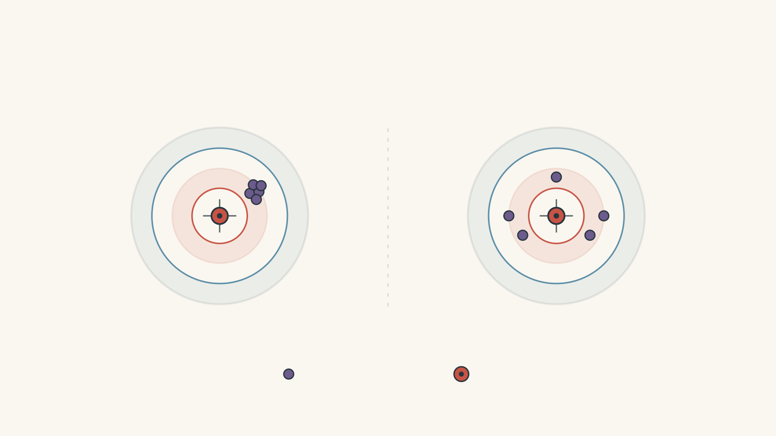
There are four possible combinations:
| Precision | Accuracy | Interpretation |
|---|---|---|
| High | High | Measurements are closely grouped and close to the accepted value. |
| High | Low | Measurements are closely grouped but consistently displaced from the accepted value. |
| Low | High | Measurements are widely scattered but their mean is close to the accepted value. |
| Low | Low | Measurements are widely scattered and their mean is far from the accepted value. |
The important point is that standard deviation primarily tells us about precision, not accuracy.
A small standard deviation does not prove that an experiment is accurate.
For example, imagine a stopwatch that consistently records every time interval 0.20 s too high.
Repeating the experiment twenty times might produce extremely similar measurements. The standard deviation could be tiny.
However, all the measurements would still contain the same systematic offset.
Averaging more readings reduces the influence of random errors. It does not remove a systematic error shared by every reading.
This distinction is particularly important when evaluating practical investigations.
07Percentage error and percentage uncertainty: which denominator?
Students frequently use the wrong denominator when calculating percentages.
The easiest way to avoid this is to identify exactly what the percentage is describing.
Percentage error
Percentage error compares the difference between an experimental result and an accepted reference value with the accepted reference value.
\[ \boxed{ \%\text{ error}= \frac{|\bar{x}-x_{\mathrm{ref}}|} {|x_{\mathrm{ref}}|}\times100 } \]
Where:
- \(\bar{x}\) is the experimental mean.
- \(x_{\mathrm{ref}}\) is the accepted or reference value.
The denominator is the accepted value.
Why?
We want to express the experimental discrepancy as a fraction of the value we are trying to measure.
For example, if an experiment gives 9.70 m/s² and the accepted value is 9.81 m/s²:
\[ \%\text{ error} = \frac{|9.70-9.81|}{9.81}\times100 \]
\[ \boxed{\%\text{ error}=1.12\%} \]
A smaller percentage error generally indicates better agreement with the accepted value.
Percentage uncertainty in the mean
Percentage uncertainty expresses the uncertainty of the experimental mean as a fraction of that mean.
\[ \boxed{ \%\text{ uncertainty} = \frac{u_{\bar{x}}}{|\bar{x}|}\times100 } \]
The denominator is now the experimental mean.
Why?
We are expressing the uncertainty relative to the size of our measured result.
This tells us how large the uncertainty is compared with the value we are reporting.
Quick comparison
| Quantity | What it describes | Denominator |
|---|---|---|
| Mean | Central value | Number of measurements, \(n\) |
| Range | Total spread | No denominator |
| Sample standard deviation | Spread around the mean | \(n-1\) |
| Standard uncertainty in mean | Precision of the estimated mean | \(\sqrt{n}\) |
| Percentage error | Difference from accepted value | Accepted value |
| Percentage uncertainty | Uncertainty relative to measured result | Experimental mean |
If you remember only one distinction from this section, remember this:
Percentage error uses the accepted value. Percentage uncertainty uses the experimental mean.
If no accepted value is available, you can still calculate the standard deviation and percentage uncertainty, but you cannot calculate percentage error.
08Common mistakes in HSC practical calculations
A few mistakes appear repeatedly when students analyse experimental data.
| Common mistake | Correct approach |
|---|---|
| Dividing by \(n\) when calculating sample standard deviation | Divide by \(n-1\). |
| Dividing standard deviation by \(n\) to find uncertainty in the mean | Divide by \(\sqrt{n}\). |
| Treating standard deviation as the uncertainty in the mean | Calculate \(s/\sqrt{n}\) separately. |
| Assuming a small standard deviation proves accuracy | Compare the mean with an accepted reference value. |
| Using the experimental mean as the denominator for percentage error | Use the accepted reference value. |
| Removing an unusual measurement simply because it differs from the others | Investigate whether there is a genuine procedural reason to exclude it. |
| Averaging measurements that are changing systematically over time | Investigate the trend before treating the readings as repeats of one fixed quantity. |
One particularly important point concerns unusual measurements.
Suppose four titrations produce 24.80 mL, 24.85 mL, 24.80 mL, and 25.40 mL.
It might be tempting to remove 25.40 mL because it increases the standard deviation.
Don’t do that automatically.
If there was a known procedural problem, such as overshooting the endpoint, you may have a valid reason to exclude that trial according to the practical method.
If there was no identifiable problem, the result should not simply be discarded because it is inconvenient.
Statistical analysis should describe the experiment honestly, not make the results look better.
11Questions and solutions
The following questions build from straightforward statistical calculations to more demanding practical analysis. Pay attention to what each statistic actually tells you, not just which formula to use.
Question 1
A student investigates a vertical spring-mass oscillator and measures its period over five independent trials.
The recorded periods are:
\[ 0.82,\quad0.80,\quad0.81,\quad 0.83,\quad0.79\text{ s} \]
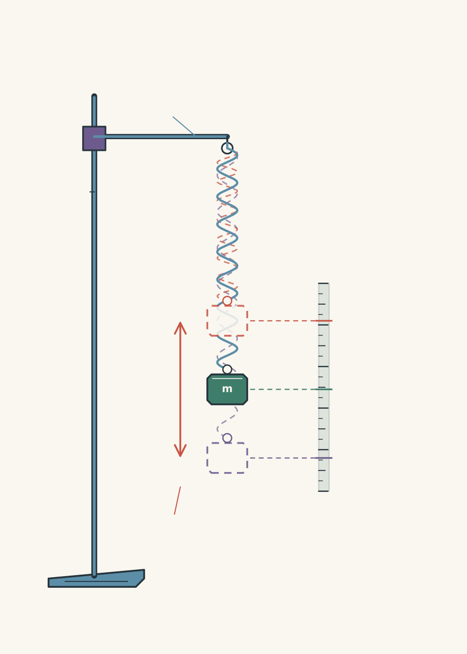
Calculate:
(a) The mean period.
(b) The range.
(c) The sample standard deviation.
(d) The standard uncertainty in the mean.
Solution 1
The mean period is 0.810 s, the range is 0.040 s, the sample standard deviation is approximately 0.0158 s, and the standard uncertainty in the mean is approximately 0.0071 s.
Step 1: Calculate the mean.
\[ \begin{aligned} \bar{x} &=\frac{0.82+0.80+0.81+0.83+0.79}{5}\\ &=\frac{4.05}{5}\\ &=0.81\text{ s} \end{aligned} \]
Step 2: Calculate the range.
\[ \text{Range}=0.83-0.79 \]
\[ \boxed{0.04\text{ s}} \]
Step 3: Calculate the sample standard deviation.
The deviations from the mean are:
\[ +0.01,\quad-0.01,\quad0,\quad +0.02,\quad-0.02 \]
The sum of their squared deviations is:
\[ \begin{aligned} \sum(x_i-\bar{x})^2 &=0.0001+0.0001\\ &\quad+0.0004+0.0004\\ &=0.0010 \end{aligned} \]
Using the sample standard deviation formula:
\[ \begin{aligned} s&=\sqrt{\frac{0.0010}{5-1}}\\ &=\sqrt{0.00025}\\ &=0.01581\text{ s} \end{aligned} \]
Step 4: Calculate the standard uncertainty in the mean.
\[ \begin{aligned} u_{\bar{x}} &=\frac{0.01581}{\sqrt{5}}\\ &=0.00707\text{ s} \end{aligned} \]
Therefore, the final result is:
\[ \boxed{T=0.810\pm0.007\text{ s}} \]
The standard deviation describes the spread of the five individual measurements, while the smaller standard uncertainty describes how precisely their mean has been determined.
Question 2
A Chemistry student performs an acid-base titration.
The preliminary rough titre is 25.10 mL. The laboratory procedure specifies that this preliminary titre must not be included in the final statistical analysis.
The three accepted titres are:
\[ 24.60,\quad24.70,\quad24.65\text{ mL} \]
The accepted reference titre is 24.80 mL.
Calculate:
(a) The mean of the accepted titres.
(b) The sample standard deviation.
(c) The standard uncertainty in the mean.
(d) The percentage error.
(e) The percentage uncertainty in the mean.
Explain why the rough titre is excluded.
Solution 2
The mean accepted titre is 24.65 mL, the sample standard deviation is 0.050 mL, and the standard uncertainty is 0.0289 mL. The percentage error is 0.60%, and the percentage uncertainty is approximately 0.12%.
Step 1: Identify the measurements to include.
The rough titre is excluded because the experimental procedure explicitly identifies it as a preliminary measurement.
We therefore use only:
\[ 24.60,\quad24.70,\quad24.65\text{ mL} \]
The rough titre is not being removed simply because it differs from the others.
Step 2: Calculate the mean.
\[ \begin{aligned} \bar{x} &=\frac{24.60+24.70+24.65}{3}\\ &=\frac{73.95}{3}\\ &=24.65\text{ mL} \end{aligned} \]
Step 3: Calculate the sample standard deviation.
The deviations from the mean are:
\[ -0.05,\quad+0.05,\quad0 \]
Their squared deviations add to:
\[ 0.0025+0.0025=0.0050 \]
Therefore:
\[ \begin{aligned} s&=\sqrt{\frac{0.0050}{3-1}}\\ &=\sqrt{0.0025}\\ &=0.050\text{ mL} \end{aligned} \]
Step 4: Calculate the standard uncertainty in the mean.
\[ \begin{aligned} u_{\bar{x}} &=\frac{0.050}{\sqrt{3}}\\ &=0.02887\text{ mL} \end{aligned} \]
Step 5: Calculate percentage error.
Use the accepted reference value as the denominator.
\[ \begin{aligned} \%\text{ error} &=\frac{|24.65-24.80|}{24.80}\times100\\ &=\frac{0.15}{24.80}\times100\\ &=0.605\% \end{aligned} \]
Step 6: Calculate percentage uncertainty.
Use the experimental mean as the denominator.
\[ \begin{aligned} \%\text{ uncertainty} &=\frac{0.02887}{24.65}\times100\\ &=0.117\% \end{aligned} \]
The final results are:
- Mean titre: 24.65 mL.
- Sample standard deviation: 0.050 mL.
- Standard uncertainty in the mean: 0.029 mL.
- Percentage error: 0.60%.
- Percentage uncertainty: 0.12%.
The important distinction is that the percentage error measures disagreement with the accepted value, while percentage uncertainty describes the uncertainty of the experimental mean.
Question 3
Two groups investigate gravitational acceleration using the same calibrated free-fall apparatus.
A steel ball is released above two light gates separated by a measured vertical distance. Each group calculates a value for gravitational acceleration from repeated trials.
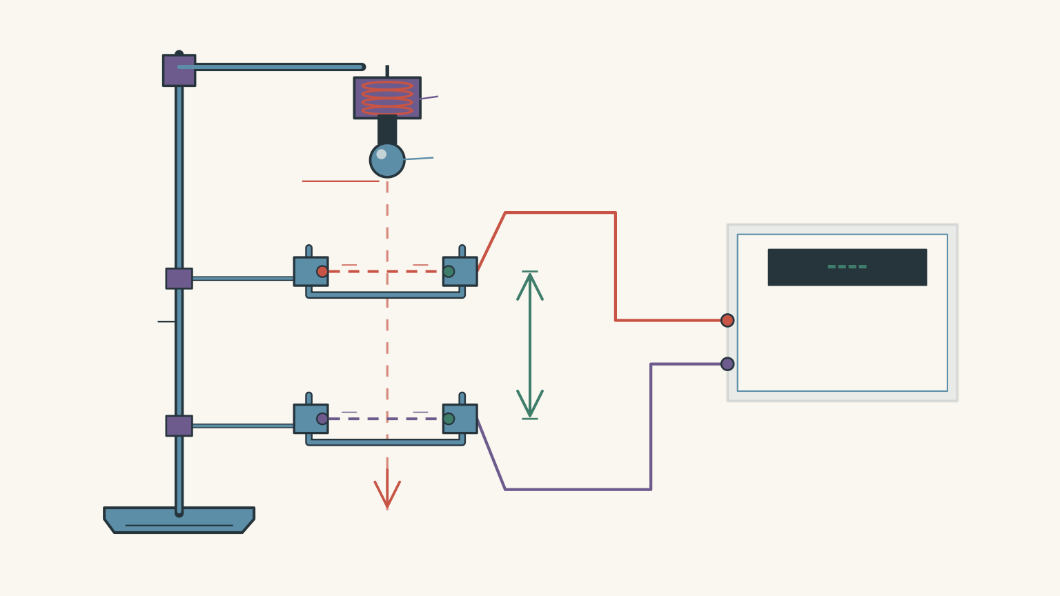
Group A obtains:
\[ 9.7,\quad9.8,\quad9.8,\quad9.9 \text{ m/s}^2 \]
Group B obtains:
\[ 9.6,\quad9.8,\quad9.8,\quad9.8, \quad9.9,\quad9.9,\quad9.8,\quad9.8 \text{ m/s}^2 \]
Use an accepted value of \(9.81\text{ m/s}^2\).
(a) Calculate the mean for each group.
(b) Calculate the sample standard deviation for each group.
(c) Calculate the standard uncertainty in the mean for each group.
(d) Which group has the smaller spread of individual measurements?
(e) Which group has the more precisely determined mean?
(f) Compare the percentage errors of the two groups.
Solution 3
Both groups obtain a mean of 9.80 m/s² and therefore have the same percentage error of approximately 0.10%. Group A has the smaller spread of individual readings, but Group B has the smaller standard uncertainty in its mean.
This is an important example of why standard deviation and standard uncertainty must be kept separate.
Step 1: Calculate the means.
For Group A:
\[ \begin{aligned} \bar{x}_A &=\frac{9.7+9.8+9.8+9.9}{4}\\ &=\boxed{9.80\text{ m/s}^2} \end{aligned} \]
For Group B:
\[ \begin{aligned} \bar{x}_B &=\frac{9.6+9.8+9.8+9.8}{} \end{aligned} \]
Including all eight readings:
\[ \begin{aligned} \bar{x}_B &=\frac{9.6+5(9.8)+2(9.9)}{8}\\ &=\frac{78.4}{8}\\ &=\boxed{9.80\text{ m/s}^2} \end{aligned} \]
Both groups obtain the same mean.
Step 2: Calculate the sample standard deviations.
For Group A, the deviations from the mean are:
\[ -0.1,\quad0,\quad0,\quad+0.1 \]
The sum of the squared deviations is:
\[ 0.01+0.01=0.02 \]
Therefore:
\[ \begin{aligned} s_A &=\sqrt{\frac{0.02}{4-1}}\\ &=\boxed{0.0816\text{ m/s}^2} \end{aligned} \]
For Group B, the deviations are:
\[ -0.2,\quad0,\quad0,\quad0,\quad +0.1,\quad+0.1,\quad0,\quad0 \]
The sum of the squared deviations is:
\[ 0.04+0.01+0.01=0.06 \]
Therefore:
\[ \begin{aligned} s_B &=\sqrt{\frac{0.06}{8-1}}\\ &=\boxed{0.0926\text{ m/s}^2} \end{aligned} \]
Group A has the smaller standard deviation.
Its individual measurements are more tightly grouped.
Step 3: Calculate the standard uncertainty in each mean.
For Group A:
\[ \begin{aligned} u_A &=\frac{0.0816}{\sqrt{4}}\\ &=\boxed{0.0408\text{ m/s}^2} \end{aligned} \]
For Group B:
\[ \begin{aligned} u_B &=\frac{0.0926}{\sqrt{8}}\\ &=\boxed{0.0327\text{ m/s}^2} \end{aligned} \]
Group B has the smaller standard uncertainty in its mean.
This happens because it has twice as many measurements. Although its individual readings are slightly more scattered, the larger sample produces a more precisely determined mean.
Step 4: Compare the percentage errors.
Both groups have the same mean, so both have the same percentage error.
\[ \begin{aligned} \%\text{ error} &=\frac{|9.80-9.81|}{9.81}\times100\\ &=0.102\% \end{aligned} \]
Therefore:
\[ \boxed{\%\text{ error}=0.10\%} \]
Both groups have the same agreement with the accepted value.
Step 5: Interpret the results.
The results demonstrate three different ideas:
- Group A has the smaller standard deviation, so its individual readings are more tightly grouped.
- Group B has the smaller standard uncertainty in the mean, so its average is more precisely determined.
- Both groups have the same percentage error, so their means agree equally well with the accepted value.
A larger sample does not necessarily produce a smaller standard deviation. It can, however, reduce the standard uncertainty in the mean.
Question 4
A Chemistry student performs a calorimetry experiment to investigate the temperature change during a reaction.
The solution is placed in an insulated polystyrene cup with a lid. A thermometer measures the temperature at regular intervals after the reactants are mixed.
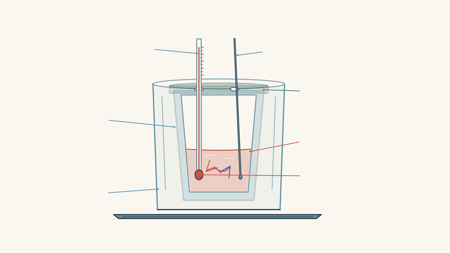
The following temperatures are recorded:
| Time after mixing (s) | Temperature (°C) |
|---|---|
| 20 | 62.0 |
| 40 | 60.8 |
| 60 | 59.6 |
| 80 | 58.4 |
| 100 | 57.2 |
A student calculates the mean and standard deviation, then reports the reaction temperature at the instant of mixing as:
\[ 59.6\pm0.85^\circ\text{C} \]
Evaluate the student’s approach.
Calculate the mean and sample standard deviation of the five readings, and estimate the temperature at the instant of mixing, assuming the cooling trend is linear over this short interval.
Solution 4
The student’s reported reaction temperature is incorrect. The mean of the five readings is 59.6°C, but these readings describe a cooling solution at different times, not repeated measurements of one constant temperature. Extrapolating the linear cooling trend back to the instant of mixing gives an estimated initial temperature of 63.2°C.
Step 1: Calculate the mean.
\[ \begin{aligned} \bar{x} &=\frac{62.0+60.8+59.6+58.4+57.2}{5}\\ &=\frac{298.0}{5}\\ &=59.6^\circ\text{C} \end{aligned} \]
The arithmetic mean is correct.
However, it represents the average of the temperatures recorded over the observation period. It does not represent the temperature at the instant of mixing.
Step 2: Calculate the sample standard deviation.
The deviations from the mean are:
\[ +2.4,\quad+1.2,\quad0,\quad-1.2,\quad-2.4 \]
The sum of the squared deviations is:
\[ \begin{aligned} \sum(x_i-\bar{x})^2 &=5.76+1.44+0\\ &\quad+1.44+5.76\\ &=14.40 \end{aligned} \]
Therefore:
\[ \begin{aligned} s&=\sqrt{\frac{14.40}{5-1}}\\ &=\sqrt{3.60}\\ &=1.90^\circ\text{C} \end{aligned} \]
The sample standard deviation is approximately 1.90°C.
The arithmetic calculation is valid as a description of the spread of these five values.
However, the temperature is clearly decreasing over time.
The measurements are not repeated observations of the same constant temperature. They represent a changing physical system.
Consequently, calculating \(s/\sqrt{5}\) would not give a meaningful standard uncertainty for the initial reaction temperature.
Step 3: Identify the cooling trend.
The temperature decreases by 1.2°C every 20 seconds.
The rate of temperature change is:
\[ \text{Rate} =\frac{60.8-62.0}{40-20} \]
\[ \text{Rate}=-0.060^\circ\text{C/s} \]
The negative sign indicates that the temperature is decreasing.
Step 4: Extrapolate back to the instant of mixing.
The first measurement was taken 20 seconds after mixing.
Over those 20 seconds, the temperature decreased by 1.2°C.
Therefore, assuming the cooling trend remains linear:
\[ T_{\mathrm{initial}}=62.0+1.2 \]
\[ \boxed{T_{\mathrm{initial}}=63.2^\circ\text{C}} \]
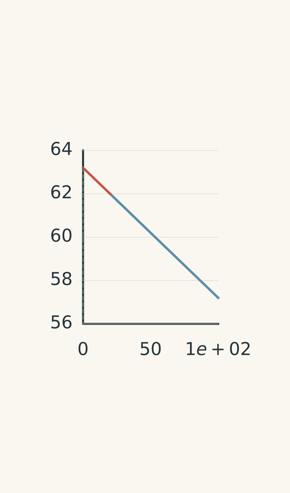
- Measured data and cooling trend
- Backward extrapolation
- Initial temperature: 63.2°C
The key lesson is that statistical calculations cannot replace understanding the physical experiment.
Before calculating a mean and standard uncertainty, check that your measurements actually represent repeated observations of the same quantity under approximately unchanged conditions.
Question 5
Two groups independently measure the period of the same pendulum by timing ten complete oscillations in each trial.
A calibrated reference system gives the accepted period:
\[ T_{\mathrm{ref}}=1.410\text{ s} \]
Team A uses an electronic timing system. A calibration test reveals that this system adds a fixed \(+0.20\text{ s}\) to every recorded ten-oscillation time.
Its five recorded total times are:
\[ 14.30,\quad14.32,\quad14.28,\quad 14.31,\quad14.29\text{ s} \]
Team B uses a calibrated manual timing method with no known fixed offset. Its five recorded total times are:
\[ 13.9,\quad14.1,\quad14.2,\quad 14.0,\quad14.3\text{ s} \]
Assume that:
- Both teams time exactly ten complete oscillations per trial.
- Team A’s fixed offset is known exactly and is the only systematic error in its timing system.
- The accepted reference period is exact for this question.
- Random measurement errors are independent between trials.
Answer the following:
(a) Calculate the uncorrected mean period for each team.
(b) Calculate the corrected mean period for Team A.
(c) Calculate the sample standard deviation of the period measurements for both teams.
(d) Calculate the standard uncertainty in the mean for both teams.
(e) Calculate the percentage error for Team A before and after applying the calibration correction. Compare it with Team B.
(f) A student argues that Team A’s very small standard deviation proves its measurements are accurate, and that taking 100 measurements would eliminate its timing offset. Explain why both claims are incorrect.
Solution 5
After applying the calibration correction, both teams obtain a mean period of 1.410 s. However, Team A has a standard uncertainty of approximately 0.00071 s, compared with 0.0071 s for Team B. Team A is therefore more precise after correction, but its uncorrected results are systematically biased.
This question tests an important interaction between random and systematic errors.
Step 1: Calculate the uncorrected mean period for Team A.
The five recorded total times are:
\[ 14.30,\quad14.32,\quad14.28,\quad 14.31,\quad14.29 \]
Their mean is:
\[ \begin{aligned} \bar{t}_A &=\frac{14.30+14.32+14.28+14.31+14.29}{5}\\ &=14.30\text{ s} \end{aligned} \]
Each measurement represents ten oscillations.
Therefore, the uncorrected mean period is:
\[ T_A=\frac{14.30}{10} \]
\[ \boxed{T_A=1.430\text{ s}} \]
Step 2: Calculate the corrected mean period for Team A.
The timing system adds 0.20 s to every recorded total time.
We must subtract this offset before calculating the corrected period.
\[ \begin{aligned} \bar{t}_{A,\mathrm{corrected}} &=14.30-0.20\\ &=14.10\text{ s} \end{aligned} \]
Divide by ten:
\[ T_{A,\mathrm{corrected}}=\frac{14.10}{10} \]
\[ \boxed{T_{A,\mathrm{corrected}}=1.410\text{ s}} \]
The corrected mean agrees with the accepted reference value.
Step 3: Calculate Team A’s sample standard deviation.
The deviations of the original total-time measurements from their mean of 14.30 s are:
\[ 0,\quad+0.02,\quad-0.02,\quad +0.01,\quad-0.01 \]
Their squared deviations add to:
\[ 0.0004+0.0004+0.0001+0.0001 =0.0010 \]
Therefore, the standard deviation of the total times is:
\[ \begin{aligned} s_{t,A} &=\sqrt{\frac{0.0010}{5-1}}\\ &=0.01581\text{ s} \end{aligned} \]
To obtain the standard deviation of the period, divide by ten:
\[ s_A=\frac{0.01581}{10} \]
\[ \boxed{s_A=0.00158\text{ s}} \]
An important mathematical property appears here.
Subtracting the same constant from every measurement changes the mean but does not change the deviations from the mean.
Therefore, correcting the fixed offset does not change the standard deviation.
Step 4: Calculate Team B’s mean period.
The recorded total times are:
\[ 13.9,\quad14.1,\quad14.2,\quad14.0,\quad14.3 \]
Their mean is:
\[ \begin{aligned} \bar{t}_B &=\frac{13.9+14.1+14.2+14.0+14.3}{5}\\ &=14.10\text{ s} \end{aligned} \]
Therefore:
\[ T_B=\frac{14.10}{10} \]
\[ \boxed{T_B=1.410\text{ s}} \]
Step 5: Calculate Team B’s sample standard deviation.
The deviations from the mean total time of 14.10 s are:
\[ -0.20,\quad0,\quad+0.10,\quad -0.10,\quad+0.20 \]
The sum of their squared deviations is:
\[ 0.04+0.01+0.01+0.04=0.10 \]
Therefore:
\[ \begin{aligned} s_{t,B} &=\sqrt{\frac{0.10}{5-1}}\\ &=\sqrt{0.025}\\ &=0.15811\text{ s} \end{aligned} \]
Convert this into the standard deviation of the period:
\[ s_B=\frac{0.15811}{10} \]
\[ \boxed{s_B=0.01581\text{ s}} \]
Team B has a much larger standard deviation than Team A.
Step 6: Calculate the standard uncertainty in each mean.
For Team A:
\[ \begin{aligned} u_A&=\frac{0.00158}{\sqrt{5}}\\ &=\boxed{0.00071\text{ s}} \end{aligned} \]
For Team B:
\[ \begin{aligned} u_B&=\frac{0.01581}{\sqrt{5}}\\ &=\boxed{0.00707\text{ s}} \end{aligned} \]
Team A has approximately one-tenth of Team B’s standard uncertainty.
After applying the correction, Team A produces the more precisely determined mean.
Step 7: Calculate percentage error.
Before correction, Team A’s mean is 1.430 s.
\[ \begin{aligned} \%\text{ error}_A &=\frac{|1.430-1.410|}{1.410}\times100\\ &=\boxed{1.42\%} \end{aligned} \]
After correction:
\[ \begin{aligned} \%\text{ error}_{A,\mathrm{corrected}} &=\frac{|1.410-1.410|}{1.410}\times100\\ &=\boxed{0.00\%} \end{aligned} \]
Team B also has a mean of 1.410 s, so its percentage error is:
\[ \boxed{\%\text{ error}_B=0.00\%} \]
Both corrected results agree with the accepted reference value.
Step 8: Evaluate the student’s claims.
The first claim is that Team A’s small standard deviation proves its measurements are accurate.
This is incorrect.
Before correction, Team A has a very small standard deviation, meaning its individual readings are tightly grouped.
However, its mean is 1.430 s rather than the accepted 1.410 s.
The measurements are precise but inaccurate because of the fixed systematic offset.
The second claim is that taking 100 measurements would eliminate the offset.
This is also incorrect.
Assuming the same random spread, increasing the number of measurements reduces the standard uncertainty in the mean:
\[ u_{\bar{x}}=\frac{s}{\sqrt{n}} \]
For Team A, if the standard deviation remains approximately 0.00158 s and the number of measurements increases to 100:
\[ \begin{aligned} u_{\bar{x}} &=\frac{0.00158}{\sqrt{100}}\\ &=\boxed{0.000158\text{ s}} \end{aligned} \]
The standard uncertainty becomes even smaller.
However, if the calibration offset is not corrected, the mean will still be approximately 1.430 s.
Taking more measurements reduces random uncertainty. It does not remove a fixed systematic error.
This is the central lesson: a result can be extremely precise and still be wrong.
12Where to go next
When analysing an HSC Physics or Chemistry practical, the first decision is whether your measurements represent repeated observations of the same quantity under unchanged conditions.
If they do, the mean, range, sample standard deviation, and standard uncertainty provide a useful description of your results.
If you are comparing your result with an accepted value, calculate percentage error separately.
Finally, remember that repeatability and accuracy require different checks. Statistical analysis describes random variation, while calibration and experimental design help identify systematic errors.
That distinction is what turns a collection of measurements into a defensible experimental result.