
Thermionic vs Photoelectric Emission: Understanding Electron Energy
Learn how thermionic and photoelectric emission differ, how work function affects electron energy, and how to interpret experimental current-voltage graphs. Includes worked examples and challenging HSC-style questions on stopping potentials, accelerating voltages, and electron energy distributions.
Imagine two evacuated tubes, each producing an electron current of 2.0 μA. In the first, electrons escape from a metal cathode because it is heated. In the second, ultraviolet light shines onto the cathode and ejects electrons.
The ammeter reads exactly the same current. Does that mean the electrons have the same kinetic energy?
No. Current tells you how much charge arrives per second. It does not tell you how much energy each electron carries. To investigate electron energy, you need to understand how the electrons were released and how they respond to an electric field.
This is the key difference between thermionic emission and photoelectric emission. Both release electrons from a metal, but they use different energy sources, produce different energy distributions, and require different approaches when interpreting experimental graphs.
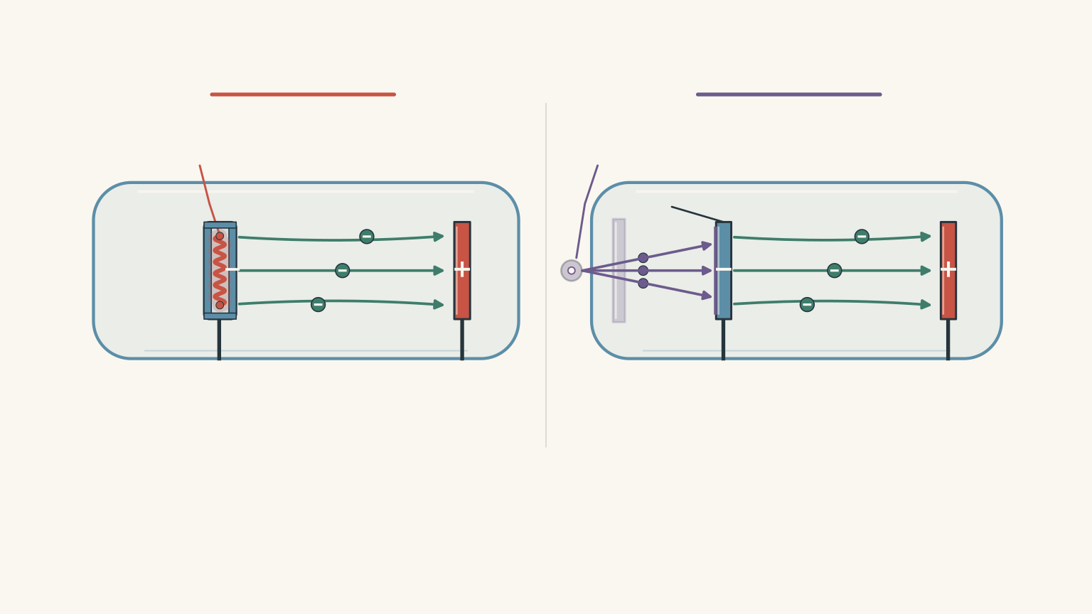
01Two ways to release an electron
Before comparing the experiments, we need one important idea: electrons inside a metal cannot simply escape into the surrounding vacuum without overcoming an energy barrier.
The work function: the energy barrier
The work function, represented by \(\phi\), is the minimum energy required to remove an electron from a metal’s surface.
It is usually measured in electronvolts (eV).
Think of the metal surface as a fence. An electron needs enough energy to get over it. The height of the fence represents the work function.
Different metals have different work functions. Even the same metal can have a different work function if its surface condition changes.
The important point is that both thermionic and photoelectric emission must overcome this same type of energy barrier.
What changes is how the electron receives the energy.
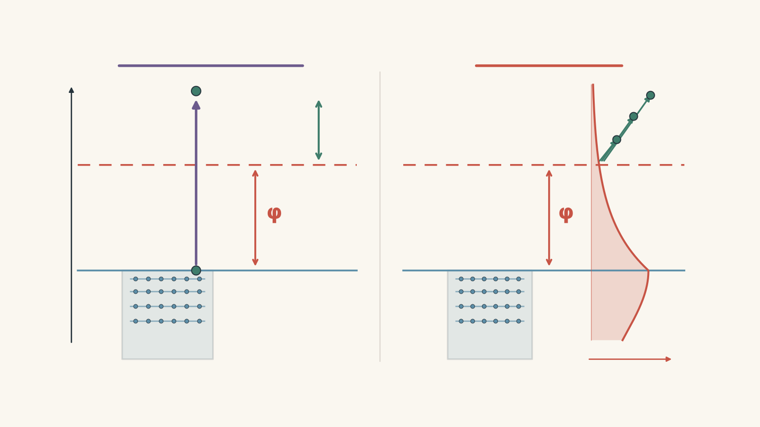
Photoelectric emission: energy from light
In photoelectric emission, an electron absorbs energy from an incoming photon.
A photon is a discrete packet of electromagnetic energy. Its energy depends on the frequency of the light:
\[ E_{\text{photon}}=hf \]
where:
- \(E_{\text{photon}}\) is the energy of one photon, in joules or electronvolts.
- \(h\) is Planck’s constant, \(6.63\times10^{-34}\,\mathrm{J\,s}\).
- \(f\) is the frequency of the light, in hertz.
If the photon does not supply enough energy to overcome the work function, the electron cannot escape through ordinary single-photon photoelectric emission.
If the photon supplies more energy than the work function, the excess becomes kinetic energy.
This gives Einstein’s photoelectric equation:
\[ \boxed{K_{\max}=hf-\phi} \]
Here, \(K_{\max}\) is the maximum kinetic energy of the emitted photoelectrons.
Notice the word maximum. Not every emitted electron has this kinetic energy. Some electrons emerge with less because of their initial energy within the metal or energy losses before escaping.
The equation describes the upper limit.
There is also a threshold frequency, \(f_0\), below which photoelectric emission does not occur:
\[ f_0=\frac{\phi}{h} \]
At the threshold frequency, the photon supplies exactly enough energy to overcome the work function. The emitted electron has zero maximum kinetic energy.
Increasing the light intensity cannot compensate for a frequency below this threshold in the ordinary one-photon model.
Thermionic emission: energy from heat
Thermionic emission works differently.
Instead of absorbing photons, electrons receive thermal energy from a heated metal.
Heating the cathode changes the distribution of electron energies inside the metal. A greater proportion of electrons can acquire enough energy to overcome the work function and escape into the surrounding vacuum.
However, heating does not give every electron the same amount of extra energy.
The emitted electrons have a spread of kinetic energies. Some leave with relatively little kinetic energy, while others leave with considerably more.
This is called an energy distribution.
A useful way to picture it is a crowd of people trying to get over a fence. Giving the crowd more energy does not make everyone jump to exactly the same height. Instead, more people can clear the fence, and the population of successful jumpers changes.
The analogy has a limit: electrons in a metal are quantum particles, not ordinary objects with classical jumping energies. Their energy distribution is governed by quantum statistics.
The distinction is important:
- Photoelectric emission has a maximum kinetic energy determined by photon frequency and work function.
- Thermionic emission produces a thermal energy distribution. Temperature alone does not specify a single maximum kinetic energy.
Do not apply \(K_{\max}=hf-\phi\) to thermionic emission. It is the photoelectric equation, not a universal equation for electrons escaping a metal.
Can temperature tell us the electron energy?
Temperature does provide a useful energy scale.
For thermal systems, this scale is given by:
\[ E_{\text{thermal}}\sim kT \]
where:
- \(k\) is Boltzmann’s constant, \(1.38\times10^{-23}\,\mathrm{J\,K^{-1}}\).
- \(T\) is the absolute temperature in kelvin.
For example, at 1200 K:
\[ \begin{aligned} kT&=(1.38\times10^{-23})(1200)\\ &=1.66\times10^{-20}\,\mathrm{J} \end{aligned} \]
Converting to electronvolts:
\[ E_{\text{thermal}} =\frac{1.66\times10^{-20}}{1.60\times10^{-19}} \]
\[ \boxed{E_{\text{thermal}}\approx0.104\,\mathrm{eV}} \]
This is a characteristic thermal energy scale. It is not the maximum kinetic energy of an emitted electron.
Electrons inside a metal also occupy a range of quantum energy states. Heating changes their occupation, and emission selects electrons capable of escaping the surface.
You might recognise \(\frac{3}{2}kT\) from the average translational kinetic energy of a classical ideal gas. It is not the maximum kinetic energy of thermionically emitted electrons, and it should not be treated as a universal thermionic emission formula.
02How the photoelectric experiment measures electron energy
The photoelectric effect became particularly interesting because early experiments produced results that classical wave theory could not adequately explain.
The experimental problem
In the late nineteenth century, Heinrich Hertz observed that ultraviolet light affected electrical discharges between metal electrodes.
Wilhelm Hallwachs subsequently demonstrated that ultraviolet light could discharge a negatively charged zinc plate. These observations suggested that light could cause negative charge to leave a metal.
But an important question remained:
How much kinetic energy did the emitted electrons actually have?
Simply observing that a metal discharged did not answer this.
Further experiments, including those by Philipp Lenard, used electric fields to investigate the energy of emitted electrons. Einstein’s photon explanation followed in 1905, and Robert Millikan later carried out precise measurements testing the predicted relationship between frequency and electron energy.
Understanding the photocell apparatus
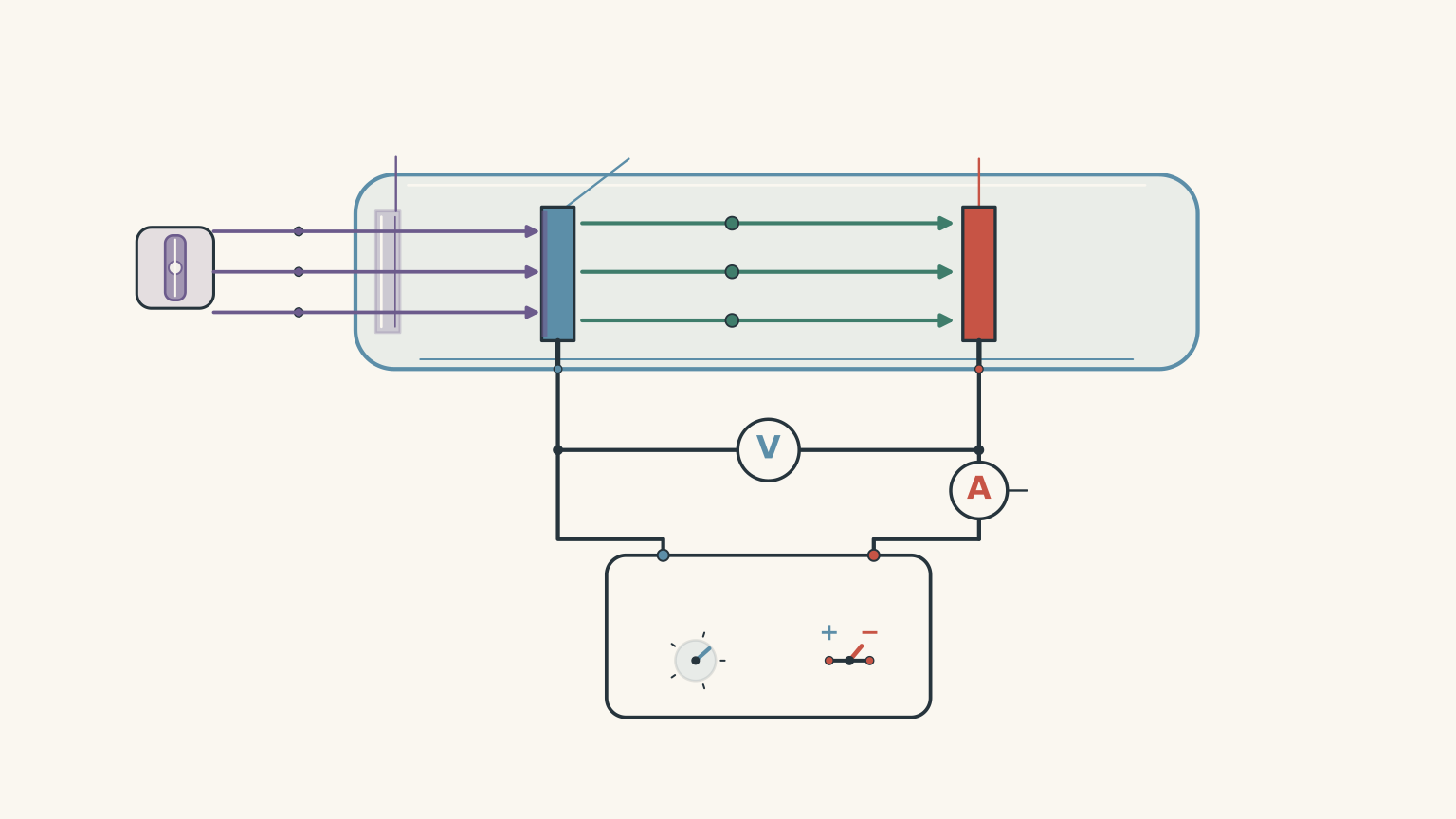
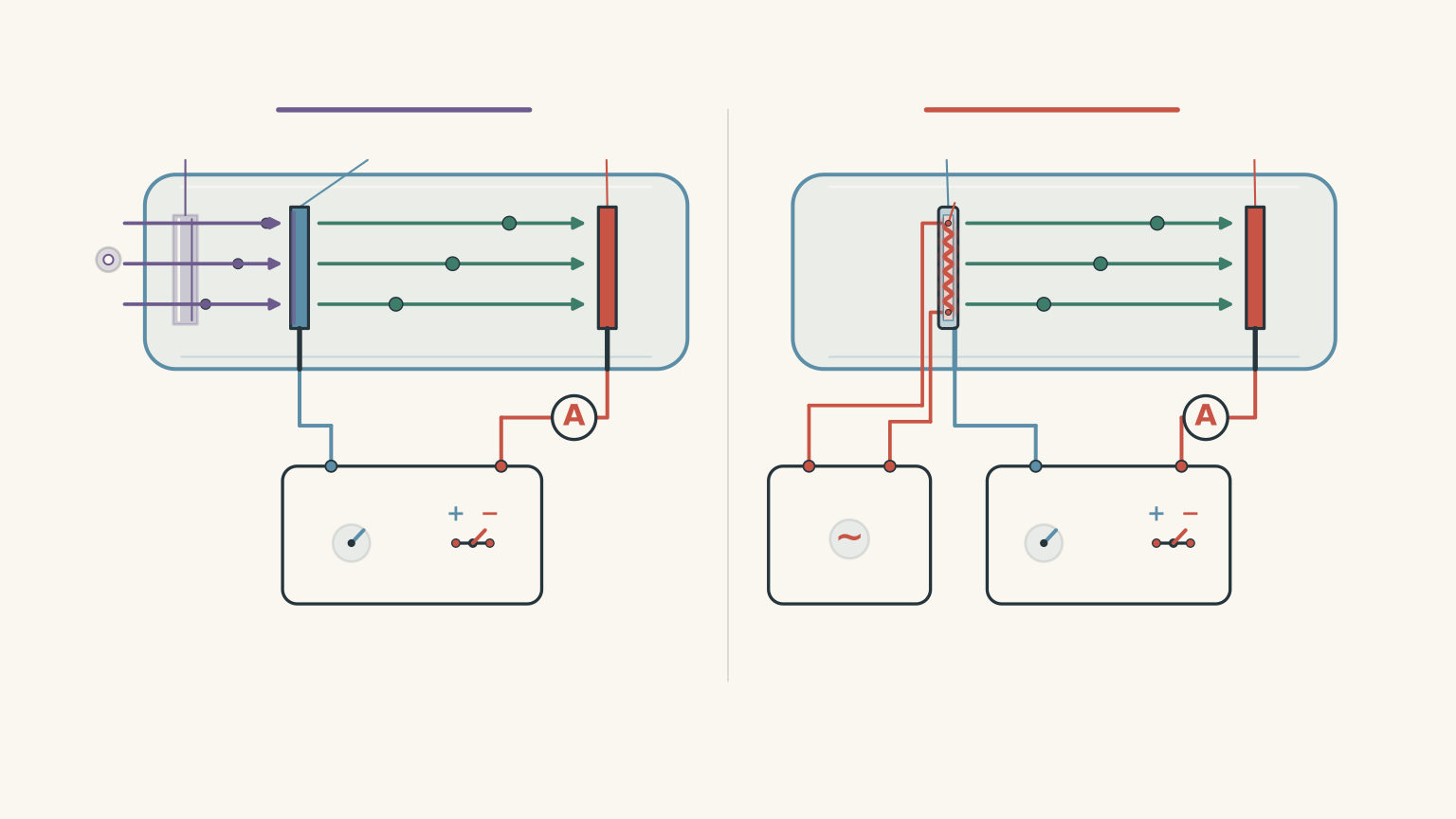
A standard photoelectric experiment uses an evacuated tube containing two metal electrodes.
The apparatus is arranged as follows:
- A photosensitive metal plate acts as the cathode.
- Light enters through a window and strikes the cathode.
- Electrons are emitted from the illuminated surface.
- A second metal plate, the anode, collects the electrons.
- An adjustable power supply controls the potential difference between the electrodes.
- An ammeter measures the resulting photocurrent, while a voltmeter measures the potential difference.
The vacuum allows electrons to travel between the electrodes without significant collisions with air molecules.
The experiment can now investigate two different things:
- How many electrons reach the anode.
- How much kinetic energy the electrons must have to reach the anode.
These are not the same measurement.
What happens when the anode is positive?
First, make the anode positive relative to the cathode.
Electrons have negative charge, so they are attracted towards the positive anode.
As the positive potential increases, more of the emitted electrons reach the collector. The measured photocurrent increases.
Eventually, the photocurrent reaches a plateau.
This is the saturation current.
At saturation, essentially all emitted electrons that can be collected are reaching the anode. Increasing the positive potential further does not significantly increase the current.
The saturation current therefore tells us about the rate of electron collection, not the kinetic energy of an individual electron.
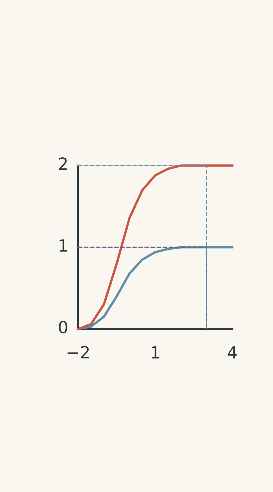
- Lower light intensity
- Higher light intensity
- Shared stopping potential
- Lower saturation current
- Higher saturation current
What happens when the anode is negative?
Now reverse the power supply so that the anode becomes negative relative to the cathode.
The anode repels the emitted electrons.
Instead of accelerating towards the collector, electrons must now use their initial kinetic energy to overcome an opposing electric field.
This is called a retarding potential.
As the magnitude of the negative potential increases, fewer electrons have enough kinetic energy to reach the anode. The photocurrent decreases.
Eventually, even the fastest electrons cannot reach the collector.
The photocurrent becomes zero.
The magnitude of the potential difference at this point is called the stopping potential, \(V_s\).
The stopping potential gives us a way to calculate the maximum kinetic energy of the photoelectrons:
\[ \boxed{K_{\max}=eV_s} \]
where \(e\) is the magnitude of the electron charge:
\[ e=1.60\times10^{-19}\,\mathrm{C} \]
The physical reasoning is simple.
At the stopping potential, the electric field removes exactly enough kinetic energy to stop the most energetic photoelectrons.
Their initial maximum kinetic energy is therefore equal to the electrical energy required to stop them.
An especially useful HSC shortcut follows:
\[ \boxed{K_{\max}(\mathrm{eV})=V_s(\mathrm{V})} \]
For example, a stopping potential of 0.80 V corresponds to a maximum kinetic energy of 0.80 eV.
This numerical shortcut works because one electronvolt is the energy transferred to an electron when it moves through a potential difference of one volt.
Worked example: Finding maximum kinetic energy from light wavelength
A metal has a work function of 2.20 eV. It is illuminated with light of wavelength 400 nm.
Calculate:
(a) the maximum kinetic energy of the emitted photoelectrons;
(b) the stopping potential;
(c) the maximum kinetic energy when the electrons reach an anode at a potential of +1.50 V relative to the cathode.
Use \(hc=1240\,\mathrm{eV\,nm}\).
Step 1
We are given wavelength rather than frequency, so use:
\[ E_{\text{photon}}=\frac{hc}{\lambda} \]
Substituting:
\[ E_{\text{photon}}=\frac{1240}{400} \]
\[ E_{\text{photon}}=3.10\,\mathrm{eV} \]
Step 2
Subtract the work function from the photon energy:
\[ K_{\max}=hf-\phi \]
\[ K_{\max}=3.10-2.20 \]
\[ \boxed{K_{\max}=0.90\,\mathrm{eV}} \]
Step 3
Using \(K_{\max}=eV_s\):
\[ \boxed{V_s=0.90\,\mathrm{V}} \]
The collector must therefore be at approximately -0.90 V relative to the cathode to stop the fastest photoelectrons.
Step 4
The anode is positive, so it accelerates the electrons.
Each electron gains 1.50 eV of kinetic energy:
\[ K_{\text{final,max}}=0.90+1.50 \]
\[ \boxed{K_{\text{final,max}}=2.40\,\mathrm{eV}} \]
The electrons originally leave the cathode with a maximum kinetic energy of 0.90 eV. After acceleration through the positive potential difference, the maximum kinetic energy becomes 2.40 eV.
Notice that the accelerating potential changes the energy measured at the anode. It does not change the original photoelectric maximum kinetic energy.
Reading a graph of stopping potential against frequency
The photoelectric experiment also allows us to investigate how maximum kinetic energy changes with light frequency.
Einstein’s equation is:
\[ K_{\max}=hf-\phi \]
Since \(K_{\max}=eV_s\):
\[ eV_s=hf-\phi \]
Rearranging:
\[ \boxed{V_s=\frac{h}{e}f-\frac{\phi}{e}} \]
This is the equation of a straight line:
\[ y=mx+c \]
Therefore, if we plot stopping potential against frequency:
- The gradient is \(h/e\).
- The vertical intercept is \(-\phi/e\).
- The horizontal intercept is the threshold frequency \(f_0\).
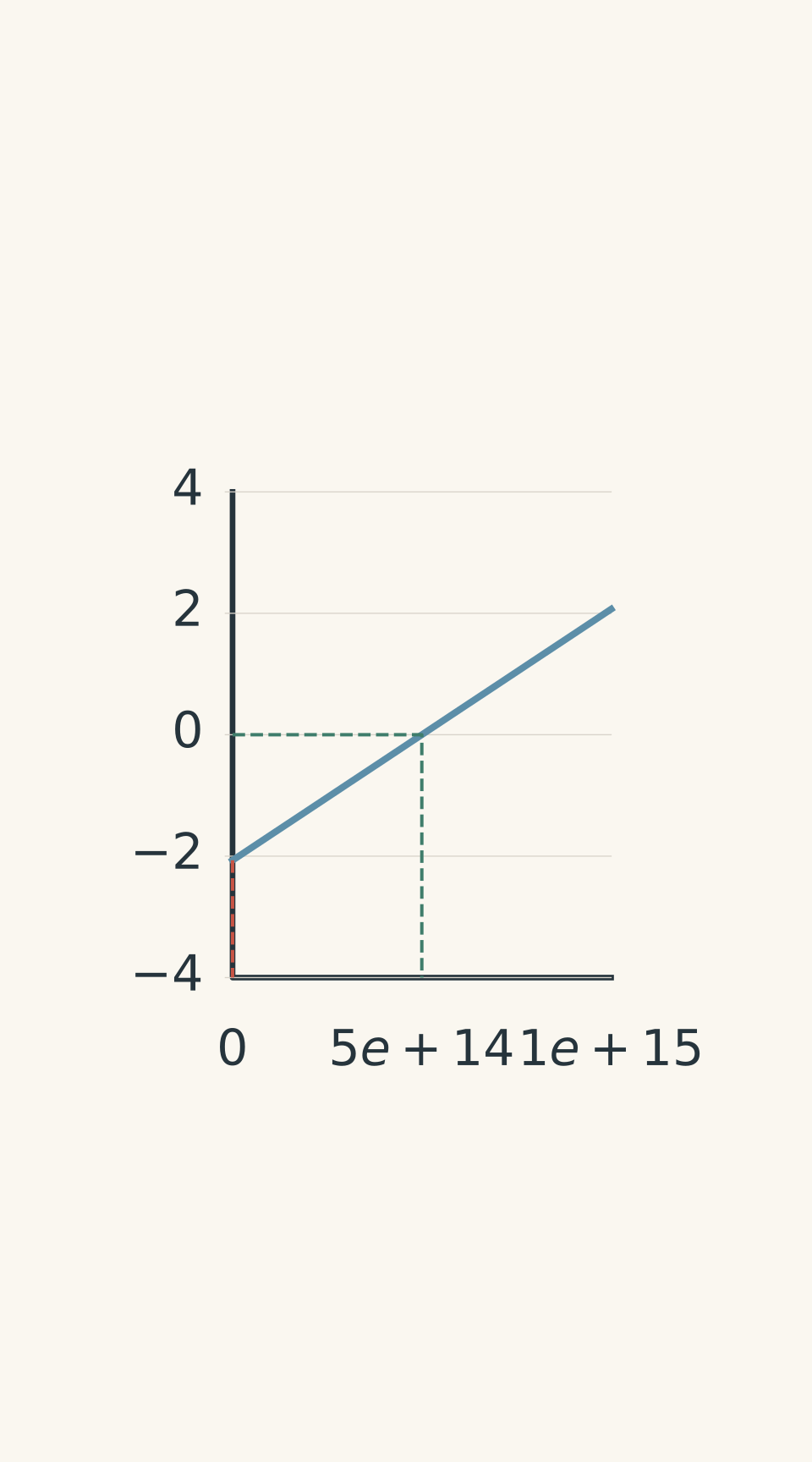
- Photoelectric line — gradient h/e
- Vertical intercept = -phi/e
- Threshold frequency f0
This graph is particularly useful because it lets us determine Planck’s constant and the work function experimentally.
Worked example: Extracting Planck’s constant from experimental data
A photocell is illuminated with light of different frequencies. The following stopping potentials are measured:
| Frequency (Hz) | Stopping potential (V) |
|---|---|
| \(6.0\times10^{14}\) | 0.48 |
| \(8.0\times10^{14}\) | 1.31 |
Assume both measurements use the same cathode surface and that contact-potential effects are negligible.
Calculate:
(a) Planck’s constant using the gradient;
(b) the work function of the metal;
(c) the threshold frequency.
Use \(e=1.60\times10^{-19}\,\mathrm{C}\).
Step 1
The gradient is the change in stopping potential divided by the change in frequency:
\[ m=\frac{\Delta V_s}{\Delta f} \]
Substituting:
\[ m=\frac{1.31-0.48} {(8.0-6.0)\times10^{14}} \]
\[ \boxed{m=4.15\times10^{-15}\,\mathrm{V\,s}} \]
Step 2
We know that:
\[ m=\frac{h}{e} \]
Therefore:
\[ h=em \]
\[ h=(1.60\times10^{-19})(4.15\times10^{-15}) \]
\[ \boxed{h=6.64\times10^{-34}\,\mathrm{J\,s}} \]
This is very close to the accepted value of Planck’s constant.
Step 3
Use the first experimental measurement.
The photon energy is:
\[ hf=(4.14\times10^{-15})(6.0\times10^{14}) \]
\[ hf=2.48\,\mathrm{eV} \]
The maximum kinetic energy is:
\[ K_{\max}=eV_s=0.48\,\mathrm{eV} \]
Rearrange Einstein’s equation:
\[ \phi=hf-K_{\max} \]
\[ \phi=2.48-0.48 \]
\[ \boxed{\phi=2.00\,\mathrm{eV}} \]
Step 4
At the threshold frequency, the maximum kinetic energy is zero:
\[ f_0=\frac{\phi}{h} \]
Using \(h=4.14\times10^{-15}\,\mathrm{eV\,s}\):
\[ f_0=\frac{2.00}{4.14\times10^{-15}} \]
\[ \boxed{f_0=4.83\times10^{14}\,\mathrm{Hz}} \]
The metal therefore requires light with a frequency of at least approximately \(4.83\times10^{14}\) Hz to produce photoelectric emission under the stated model.
03How thermionic experiments measure electron energy
Thermionic emission experiments use a similar evacuated tube, but the source of the electrons is different.
Instead of shining light onto the cathode, we heat it.
Understanding the thermionic diode
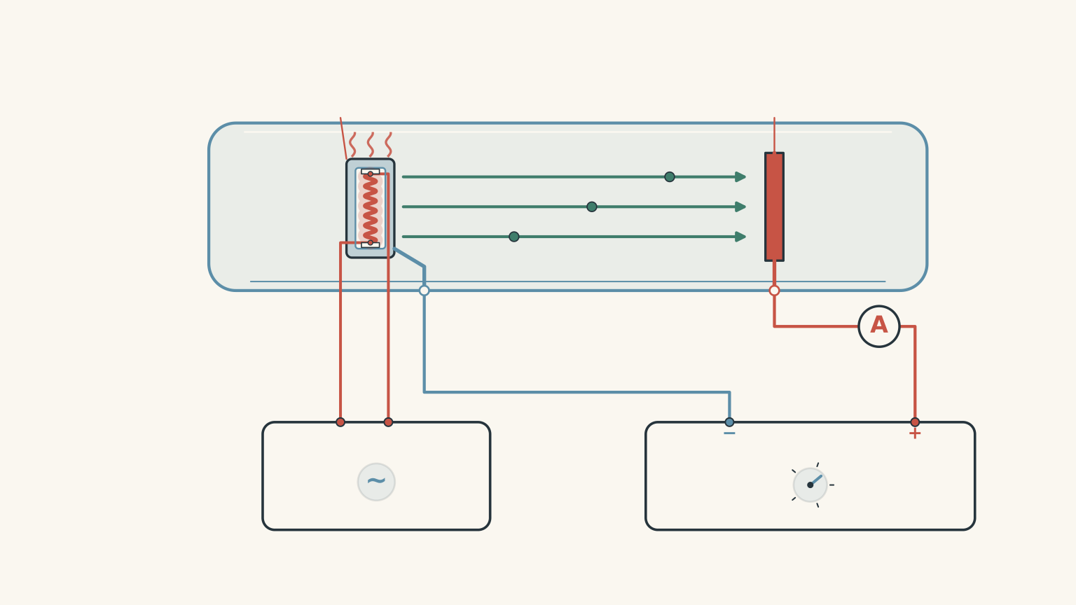
A typical thermionic diode contains:
- A heated metal cathode, which releases electrons.
- An anode, which collects the electrons.
- A separate heater circuit, which controls cathode temperature.
- An adjustable anode supply, which controls the electric field.
- An ammeter, which measures the current through the tube.
The cathode is heated using a separate electrical circuit. This distinction is important.
The heater circuit controls the temperature of the cathode. The anode supply controls the potential difference that accelerates or retards the emitted electrons.
These are two different controls.
What happens when the anode is positive?
When the anode is positive relative to the cathode, it attracts the electrons released by heating.
As the positive potential increases, more electrons are collected.
Eventually, the current reaches a saturation value.
At this point, essentially all available emitted electrons are being collected.
Now increase the cathode temperature.
What should happen to the saturation current?
It increases.
A hotter cathode allows a greater number of electrons to overcome the work function and escape. More electrons are available for collection, so the current increases.
This means thermionic saturation current is strongly affected by cathode temperature.
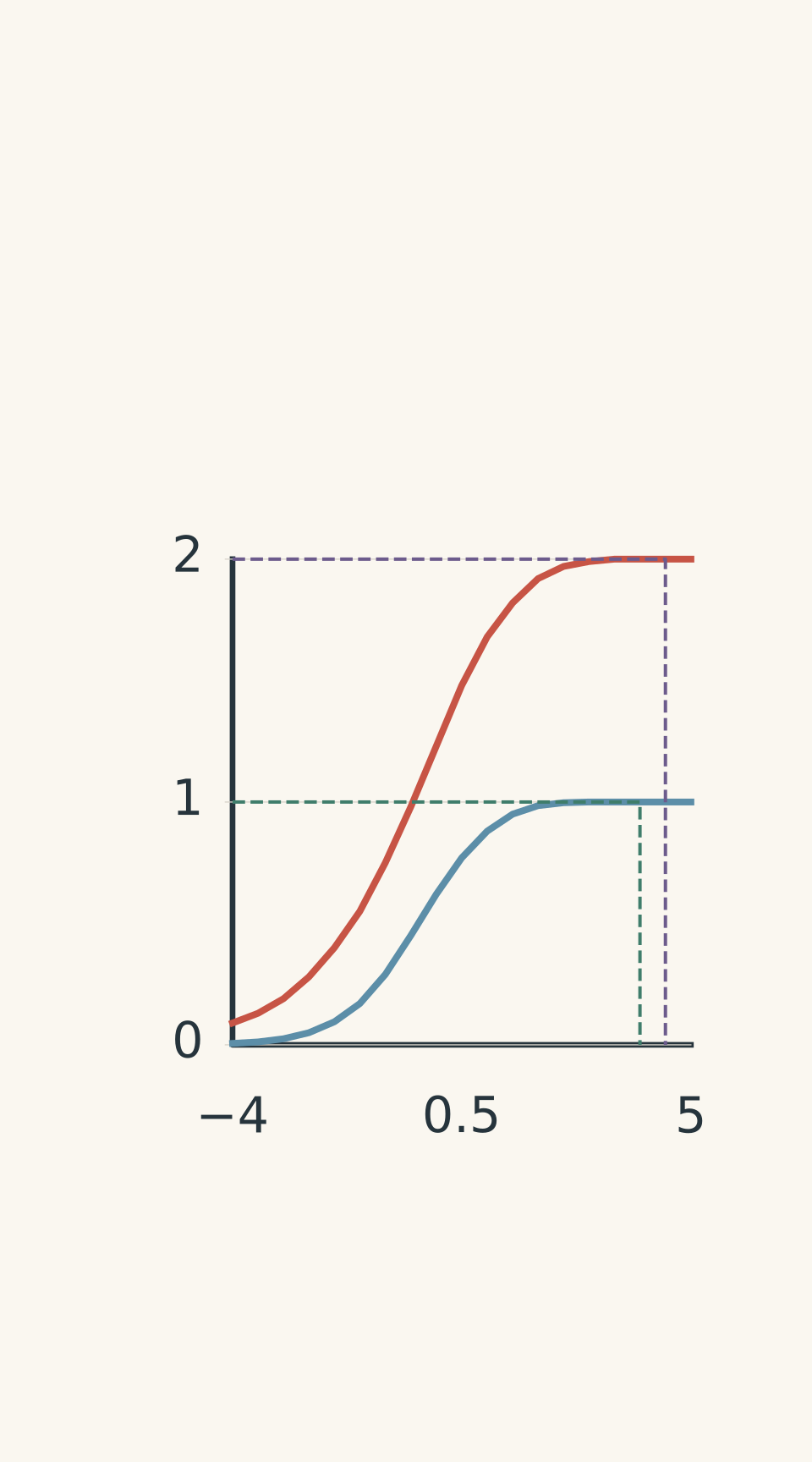
- Cooler cathode (lower temperature)
- Hotter cathode (higher temperature)
- Cooler saturation
- Hotter saturation
What happens when the anode is negative?
The anode now repels the electrons, just as it did in the photoelectric experiment.
However, there is an important difference in how we interpret the resulting graph.
Thermionically emitted electrons have a distribution of kinetic energies.
Some electrons are relatively slow. Others have enough kinetic energy to overcome a stronger retarding potential.
As the magnitude of the negative anode potential increases, the slower electrons are turned back first. Faster electrons continue to reach the collector.
Consequently, the current decreases progressively.
A retarding-potential experiment therefore gives information about the distribution of electron energies.
It does not give a single universal maximum kinetic energy based on temperature alone.
In fact, the highest energy observed in a thermionic experiment depends on the population of emitted electrons, the measurement time, the surface conditions, and the sensitivity of the apparatus.
A sufficiently rare high-energy electron might not be detected at all.
Why the thermionic graph is not the same as the photoelectric graph
Both experiments use a retarding potential to filter electrons according to their kinetic energy.
However, the energy of photoelectrons has a specific maximum predicted by Einstein’s equation:
\[ K_{\max}=hf-\phi \]
For thermionic emission, the electrons emerge with a thermal energy distribution.
There is no equivalent equation that allows you to substitute temperature for photon frequency and calculate a unique \(K_{\max}\).
Temperature changes the distribution and the number of electrons emitted. It does not establish a sharp, universal upper energy limit.
This distinction is particularly important when analysing a graph.
If a thermionic current becomes too small to measure at a retarding potential of 1.0 V, you can conclude that the number of electrons reaching the collector above that energy threshold is below the apparatus’s detection limit.
You cannot automatically conclude that the maximum kinetic energy of every emitted electron is exactly 1.0 eV.
What happens in an electron gun?
Thermionic emission is commonly used in electron guns.
A heated cathode supplies electrons, while an accelerating potential gives those electrons additional kinetic energy.
For an electron moving through a potential difference, the change in kinetic energy is:
\[ \boxed{\Delta K=e\Delta V} \]
Here, \(\Delta V\) is the final electric potential minus the initial electric potential.
Because the electron has charge \(-e\), moving towards a higher electric potential increases its kinetic energy.
If the accelerating voltage is large compared with the initial thermal kinetic energies, the final beam energy is approximately:
\[ K\approx eV_{\text{acc}} \]
where \(V_{\text{acc}}\) is the accelerating potential difference.
This is an approximation, not an exact statement that every electron leaves the cathode with zero kinetic energy.
The initial energy distribution is still present after acceleration. The accelerating voltage shifts the energies of the electrons upwards, rather than making them all identical.
04Comparing thermionic and photoelectric emission
The two mechanisms are easier to distinguish when their experimental behaviour is placed side by side.
| Feature | Photoelectric emission | Thermionic emission |
|---|---|---|
| Energy source | Photons | Thermal energy |
| How electrons escape | Absorb photon energy | Acquire sufficient thermal energy |
| Role of work function | Minimum energy required to escape | Minimum energy barrier to escape |
| Main control of emission rate | Light intensity at fixed frequency | Cathode temperature |
| Main control of maximum energy | Light frequency | No single maximum determined by temperature alone |
| Energy distribution | A range of energies with a defined maximum | A thermal distribution |
| Positive anode potential | Accelerates electrons | Accelerates electrons |
| Negative anode potential | Retards electrons and allows measurement of stopping potential | Filters electrons according to their kinetic energies |
| Relevant energy relationship | \(K_{\max}=hf-\phi\) | No equivalent universal \(K_{\max}(T)\) equation |
A final distinction: current versus energy
When interpreting either experiment, separate three different quantities.
1. Emission rate
How many electrons leave the cathode each second?
This is related to the measured current.
The relationship is:
\[ I=\frac{Q}{t} \]
where \(I\) is current, \(Q\) is charge, and \(t\) is time.
If \(N\) electrons are collected each second:
\[ I=Ne \]
2. Electron kinetic energy
How much kinetic energy does an individual electron carry?
This is determined by the emission mechanism and any applied potential difference.
3. Energy distribution
Do all emitted electrons have the same kinetic energy, or is there a range?
This determines how the current responds when a retarding potential is applied.
A useful exam habit is to identify which of these three quantities the question is actually asking about before selecting an equation.
05Questions and solutions
The following questions build from basic photoelectric calculations to interpreting experimental data from both emission mechanisms. The final question combines energy distributions, current measurements, and the limitations of experimental evidence.
Question 1
A metal has a work function of 2.50 eV. It is illuminated with monochromatic light of wavelength 350 nm.
Assume all emitted electrons are collected when the anode is sufficiently positive.
(a) Calculate the energy of each incoming photon.
(b) Calculate the maximum kinetic energy of the emitted photoelectrons.
(c) Determine the stopping potential.
(d) The light intensity is doubled without changing its frequency. Explain what happens to the saturation current and stopping potential.
Use \(hc=1240\,\mathrm{eV\,nm}\).
Solution 1
The maximum kinetic energy is 1.04 eV, and the stopping potential is approximately 1.04 V. Doubling the light intensity increases the saturation current but does not change the stopping potential.
(a) Calculate photon energy.
Use:
\[ E_{\text{photon}}=\frac{hc}{\lambda} \]
Substituting:
\[ E_{\text{photon}}=\frac{1240}{350} \]
\[ \boxed{E_{\text{photon}}=3.54\,\mathrm{eV}} \]
(b) Calculate maximum kinetic energy.
Einstein’s photoelectric equation is:
\[ K_{\max}=hf-\phi \]
Substituting the photon energy and work function:
\[ K_{\max}=3.54-2.50 \]
\[ \boxed{K_{\max}=1.04\,\mathrm{eV}} \]
The photon supplies 3.54 eV, of which 2.50 eV is required to overcome the work function.
The remaining energy becomes kinetic energy.
(c) Calculate stopping potential.
Use:
\[ K_{\max}=eV_s \]
When kinetic energy is expressed in eV, the numerical value of the stopping potential in volts is the same:
\[ \boxed{V_s=1.04\,\mathrm{V}} \]
(d) Explain the effect of doubling intensity.
Doubling the intensity increases the number of photons arriving per second, assuming the frequency remains constant.
This increases the number of photoelectrons emitted per second and therefore increases the saturation current.
However, each photon still carries exactly the same energy because its frequency has not changed.
Therefore:
- Saturation current increases.
- Maximum kinetic energy remains unchanged.
- Stopping potential remains unchanged.
The common mistake is to assume that more intense light produces more energetic individual photoelectrons. It produces more photons per second, not more energy per photon.
Question 2
A photocell is tested using three different light conditions. The cathode material and electrode geometry remain unchanged.
The measured current-voltage data are summarised below.
| Curve | Light conditions | Saturation current | Stopping potential |
|---|---|---|---|
| A | Frequency \(f\), intensity \(I\) | 1.5 μA | 0.60 V |
| B | Frequency \(f\), intensity \(3I\) | 4.5 μA | 0.60 V |
| C | Higher frequency than B, adjusted intensity | 4.5 μA | 1.00 V |
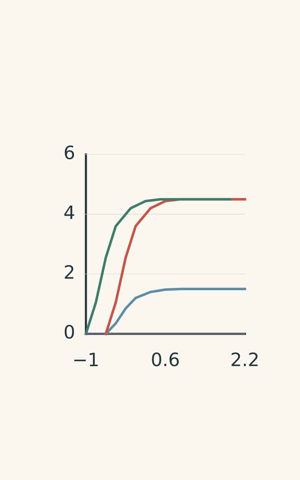
- A — saturation 1.5 μA
- B — saturation 4.5 μA
- C — saturation 4.5 μA
- A and B: stopping potential -0.60 V
- C: stopping potential -1.00 V
(a) Which two curves demonstrate the effect of changing light intensity without changing frequency?
(b) Calculate the maximum kinetic energy of the photoelectrons for each curve.
(c) Calculate the increase in light frequency between curves B and C.
(d) Explain why curves B and C can have the same saturation current but different maximum kinetic energies.
Use \(h=4.14\times10^{-15}\,\mathrm{eV\,s}\).
Solution 2
Curves A and B demonstrate the effect of intensity. Curve C produces more energetic photoelectrons than curve B, even though their saturation currents are identical. The frequency increases by approximately \(9.66\times10^{13}\) Hz.
(a) Identify the intensity comparison.
Curves A and B have the same frequency but different intensities.
The intensity of B is three times that of A.
The saturation current also increases by a factor of three:
\[ \frac{4.5}{1.5}=3 \]
This is consistent with the increased photon arrival rate producing more photoelectrons per second.
The stopping potential remains unchanged because the photon frequency has not changed.
(b) Calculate maximum kinetic energies.
Use:
\[ K_{\max}=eV_s \]
For curve A:
\[ \boxed{K_{\max,A}=0.60\,\mathrm{eV}} \]
For curve B:
\[ \boxed{K_{\max,B}=0.60\,\mathrm{eV}} \]
For curve C:
\[ \boxed{K_{\max,C}=1.00\,\mathrm{eV}} \]
Curve C produces electrons with a greater maximum kinetic energy.
(c) Calculate the frequency increase.
Einstein’s equation is:
\[ K_{\max}=hf-\phi \]
Because the cathode material is unchanged, the work function is constant.
Subtracting the equations for B and C gives:
\[ \Delta K_{\max}=h\Delta f \]
Therefore:
\[ \Delta f=\frac{\Delta K_{\max}}{h} \]
Substituting:
\[ \Delta f=\frac{1.00-0.60}{4.14\times10^{-15}} \]
\[ \boxed{\Delta f=9.66\times10^{13}\,\mathrm{Hz}} \]
The frequency has increased by approximately \(9.66\times10^{13}\) Hz.
(d) Explain the equal saturation currents.
The saturation current measures the rate at which electrons are collected.
It does not directly measure their kinetic energy.
Curves B and C have equal saturation currents, so they have equal collected electron rates under the experimental assumptions.
However, curve C has a higher stopping potential, meaning its fastest photoelectrons have greater kinetic energy.
The light intensity for C has been adjusted to give the same electron collection rate as B, despite the different photon frequency.
This demonstrates why saturation current and maximum kinetic energy must be treated as separate measurements.
Question 3
A thermionic diode is tested with its cathode at two different temperatures: 1000 K and 1400 K.
The experimental current-voltage graph shows the following behaviour:
- At 1000 K, the saturation current is 1.0 μA.
- At 1400 K, the saturation current is 5.0 μA.
- The hotter cathode also produces a greater current at the same negative retarding potential.
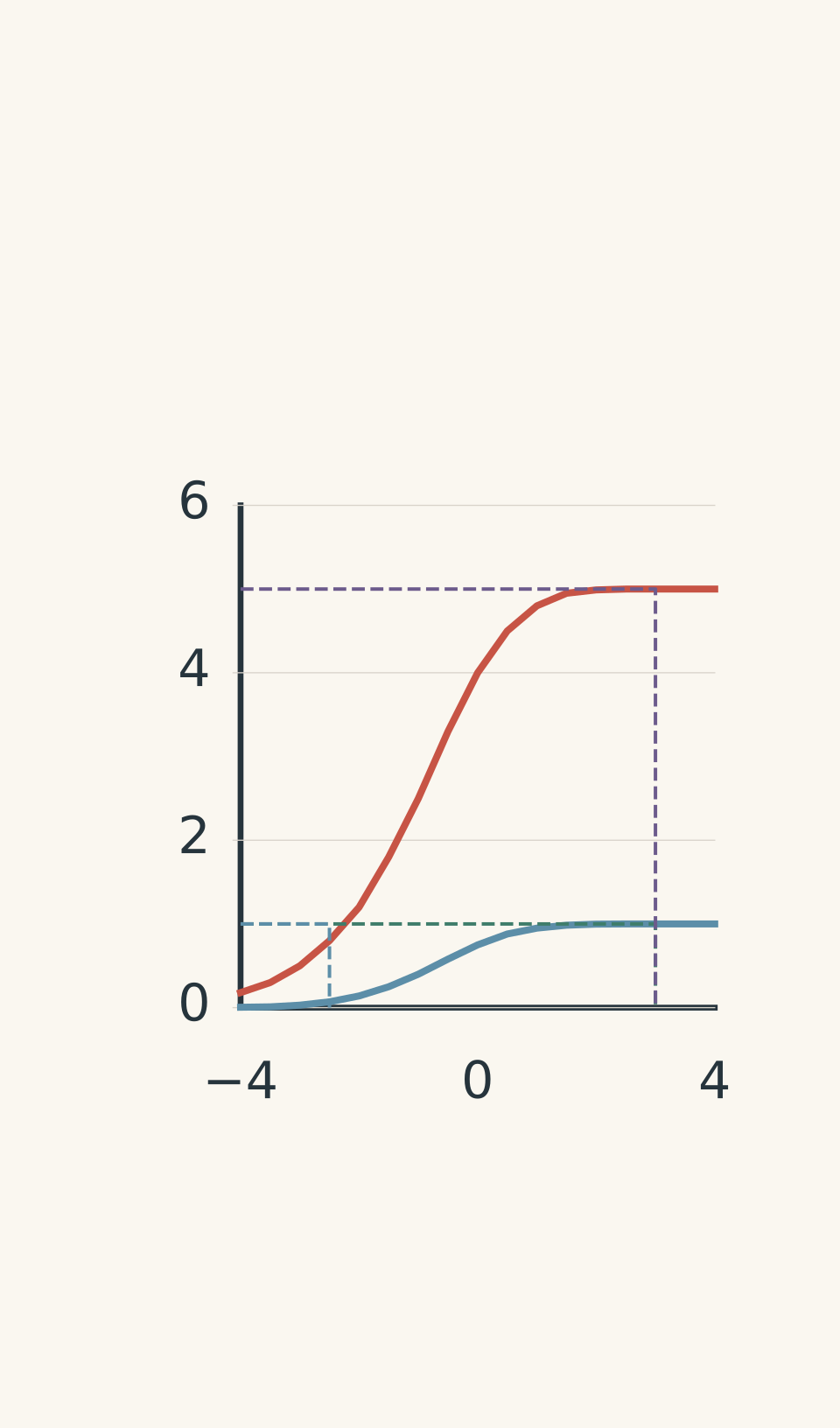
- Cooler cathode: 1000 K
- Hotter cathode: 1400 K
- 1000 K saturation: 1.0 μA
- 1400 K saturation: 5.0 μA
- Retarding region
A student makes the following claim:
“The maximum kinetic energy of the electrons at 1400 K is \(\frac{3}{2}kT\). Increasing the temperature therefore increases the maximum electron energy in direct proportion to temperature.”
(a) Explain what the increase in saturation current tells us.
(b) Explain what the greater current under a retarding potential tells us.
(c) Calculate \(kT\) at 1400 K in electronvolts.
(d) Evaluate the student’s claim.
Use \(k=1.38\times10^{-23}\,\mathrm{J\,K^{-1}}\).
Solution 3
The hotter cathode emits more electrons and produces a different energy distribution. However, its maximum kinetic energy cannot be calculated using \(\frac{3}{2}kT\).
(a) Interpret the saturation current.
The saturation current increases from 1.0 μA to 5.0 μA.
This is an increase by a factor of five.
The higher temperature allows more electrons to overcome the work function and escape from the cathode.
Since the positive anode collects these electrons, the increased emission rate produces a greater saturation current.
(b) Interpret the retarding-potential behaviour.
A greater current at the same negative potential means that more electrons have sufficient forward kinetic energy to overcome the opposing electric field.
The hotter cathode therefore produces a larger population of electrons capable of passing through the retarding field.
This provides evidence about the electron energy distribution.
It does not establish a precise maximum kinetic energy.
(c) Calculate the thermal energy scale.
Use:
\[ E_{\text{thermal}}\sim kT \]
Substituting:
\[ kT=(1.38\times10^{-23})(1400) \]
\[ kT=1.932\times10^{-20}\,\mathrm{J} \]
Convert to electronvolts:
\[ kT=\frac{1.932\times10^{-20}}{1.60\times10^{-19}} \]
\[ \boxed{kT\approx0.121\,\mathrm{eV}} \]
For comparison:
\[ \frac{3}{2}kT\approx0.181\,\mathrm{eV} \]
(d) Evaluate the claim.
The student’s conclusion is incorrect.
The expression \(\frac{3}{2}kT\) describes the average translational kinetic energy of a classical ideal gas in three dimensions.
It is not the maximum kinetic energy of thermionically emitted electrons.
Electrons inside a metal occupy a distribution of quantum energy states. Heating changes the distribution and increases the number of electrons capable of escaping the surface.
There is no universal maximum kinetic energy that can be calculated from temperature alone.
The correct interpretation is that increasing temperature increases the emission rate and changes the distribution of emitted electron energies.
Question 4
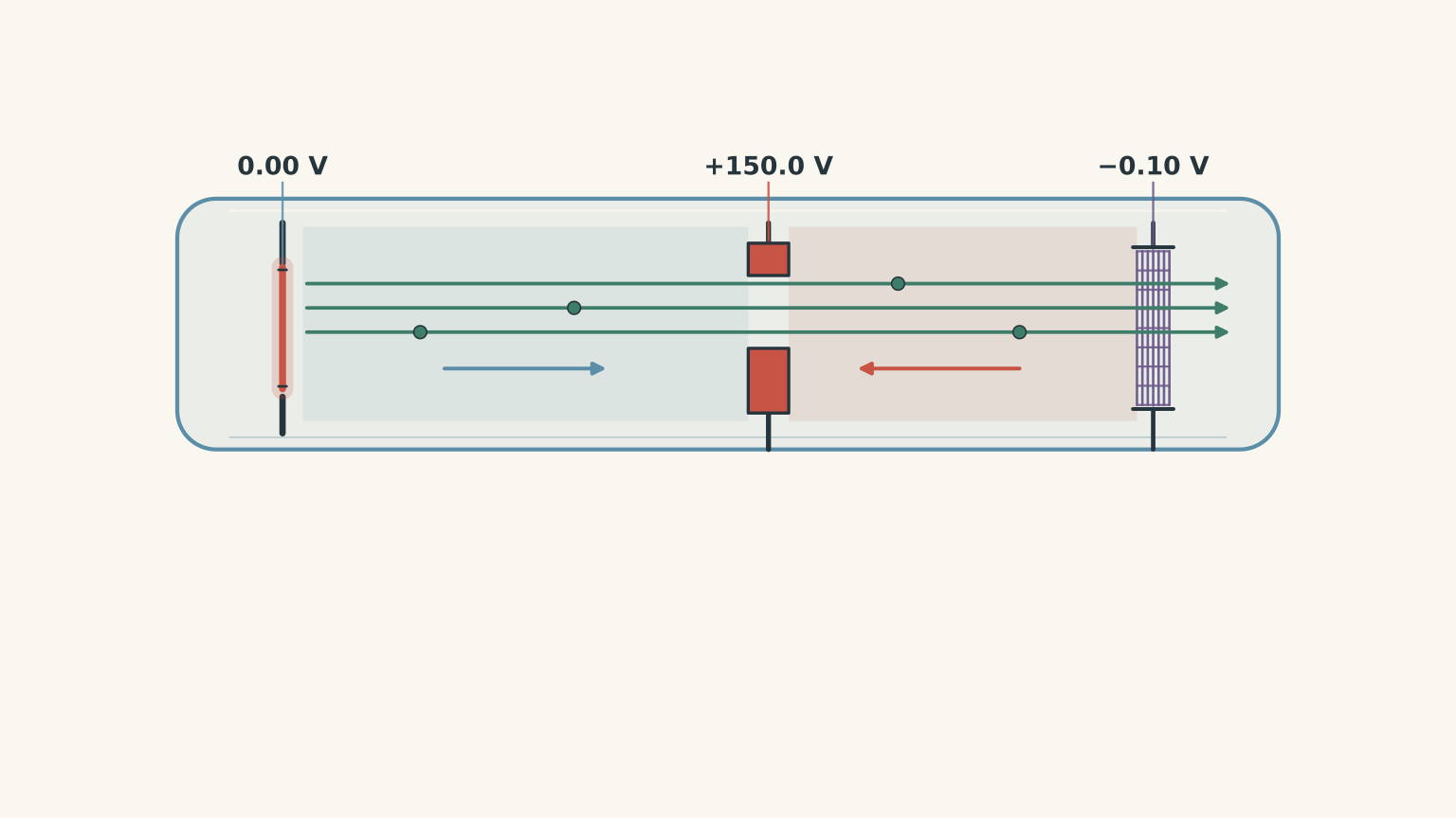
A thermionic electron gun contains a cathode, an accelerating anode, and a downstream retarding grid.
The cathode is at 0.00 V, the anode is at +150.0 V, and the retarding grid is at -0.10 V relative to the cathode.
The electrons initially emitted towards the anode have a measured forward kinetic-energy distribution that is uniform between 0.04 eV and 0.24 eV.
Assume that:
- All electrons initially travel towards the anode.
- The stated distribution is uniform in kinetic energy.
- Contact potentials and collisions are negligible.
- The retarding grid acts as an ideal energy filter.
(a) Calculate the range of kinetic energies at the accelerating anode.
(b) Determine the minimum initial kinetic energy required for an electron to pass through the retarding grid.
(c) Calculate the fraction of emitted electrons that pass through the grid.
(d) Determine the range of kinetic energies of the electrons that successfully reach the grid.
(e) Explain why the accelerating voltage does not guarantee that every electron reaches the final grid with 150 eV of kinetic energy.
Solution 4
The electrons reach the accelerating anode with energies between 150.04 eV and 150.24 eV. However, only 70% pass through the downstream retarding grid, and their final kinetic energies range from approximately 0 to 0.14 eV.
(a) Calculate the kinetic-energy range at the anode.
The anode is at +150.0 V relative to the cathode.
The electrons gain 150.0 eV of kinetic energy.
Therefore:
\[ K_{\text{anode}}=K_{\text{initial}}+150.0 \]
For the lowest-energy electrons:
\[ K_{\text{anode,min}}=0.04+150.0 \]
\[ K_{\text{anode,min}}=150.04\,\mathrm{eV} \]
For the highest-energy electrons:
\[ K_{\text{anode,max}}=0.24+150.0 \]
\[ K_{\text{anode,max}}=150.24\,\mathrm{eV} \]
Therefore:
\[ \boxed{150.04\leq K_{\text{anode}}\leq150.24\,\mathrm{eV}} \]
The original energy spread has been shifted upwards by 150 eV. It has not disappeared.
(b) Determine the minimum initial kinetic energy required.
The final grid is at -0.10 V relative to the cathode.
Therefore, an electron loses 0.10 eV of kinetic energy relative to its initial state.
An electron must initially have more than 0.10 eV to reach the grid with positive kinetic energy.
Thus:
\[ \boxed{K_{\text{initial}}>0.10\,\mathrm{eV}} \]
Electrons with initial kinetic energies below 0.10 eV are turned back before reaching the grid.
(c) Calculate the fraction that passes through.
The original distribution extends from 0.04 eV to 0.24 eV.
Its total energy range is:
\[ \Delta K=0.24-0.04 \]
\[ \Delta K=0.20\,\mathrm{eV} \]
The electrons that pass have initial energies from 0.10 eV to 0.24 eV.
The transmitted energy range is:
\[ \Delta K_{\text{pass}}=0.24-0.10 \]
\[ \Delta K_{\text{pass}}=0.14\,\mathrm{eV} \]
Because the distribution is uniform:
\[ \text{Fraction passing} =\frac{0.14}{0.20} \]
\[ \boxed{\text{Fraction passing}=0.70=70\%} \]
(d) Calculate the final kinetic-energy range.
The grid is at -0.10 V relative to the cathode.
Therefore:
\[ K_{\text{grid}}=K_{\text{initial}}-0.10 \]
For the electrons just able to pass:
\[ K_{\text{grid,min}}\approx0\,\mathrm{eV} \]
For the fastest electrons:
\[ K_{\text{grid,max}}=0.24-0.10 \]
\[ K_{\text{grid,max}}=0.14\,\mathrm{eV} \]
Therefore:
\[ \boxed{0\leq K_{\text{grid}}\leq0.14\,\mathrm{eV}} \]
The zero-energy endpoint represents the limiting electron that just reaches the grid.
(e) Explain the role of the two potentials.
The tempting conclusion is that an electron accelerated through 150 V must permanently retain 150 eV of additional kinetic energy.
But the electric field can also remove kinetic energy.
The electrons first gain 150 eV travelling from the cathode to the anode. They then encounter a strong retarding field as the potential falls from +150.0 V to -0.10 V.
The net potential change from cathode to grid is only -0.10 V.
Consequently, the final kinetic energy depends on the original kinetic energy minus 0.10 eV.
This is an application of energy conservation: the intermediate acceleration does not determine the final energy independently of the subsequent retarding field.
Question 5
Two evacuated electron-emission devices are connected to identical retarding-potential analysers.
Device P uses photoelectric emission from a metal illuminated with monochromatic light.
Device T uses thermionic emission from a heated cathode.
Both devices have the same electrode geometry and reach a saturation current of 4.00 μA when the collector is sufficiently positive.
Their currents are then measured at different negative collector potentials.
| Collector potential | Photoelectric device P | Thermionic device T |
|---|---|---|
| +5.00 V | 4.00 μA | 4.00 μA |
| -0.40 V | 3.00 μA | 2.00 μA |
| -0.80 V | Below 0.01 μA | 0.50 μA |
| -1.20 V | Below 0.01 μA | Below 0.01 μA |
A finer measurement of device P places its stopping potential at \(0.78\pm0.02\) V.
Assume:
- All electrons initially travel towards the collector.
- The retarding potential filters electrons according to their forward kinetic-energy component.
- The measured current is proportional to the number of electrons that pass the retarding field.
- The apparatus cannot reliably measure currents below 0.01 μA.
(a) Calculate the number of electrons collected per second by each device at saturation.
(b) At a retarding potential of -0.40 V, calculate the percentage of electrons passing through each device.
(c) What percentage of the thermionic electrons have sufficient forward kinetic energy to pass through a retarding potential of -0.80 V?
(d) Compare the energy distributions of the two devices. What can be inferred from the measurements at -0.80 V and -1.20 V?
(e) A student argues:
“Both devices have the same saturation current, so they must produce the same electron energy distribution. Also, because neither device produces measurable current at -1.20 V, both must have a maximum kinetic energy of exactly 1.20 eV.”
Evaluate both statements.
(f) Suppose the complete ideal retarding-current curves of the two devices were identical at every possible retarding potential, not just at the three measured values. Would this prove that the two devices used the same emission mechanism? Explain carefully.
Solution 5
Both devices collect approximately \(2.50\times10^{13}\) electrons per second at saturation, but their energy distributions are different. Equal saturation currents do not imply equal electron energies, and the absence of measurable current at a particular retarding potential does not establish an exact maximum kinetic energy.
(a) Calculate the electron collection rate.
At saturation, both devices have a current of:
\[ I=4.00\times10^{-6}\,\mathrm{A} \]
The magnitude of the charge on one electron is:
\[ e=1.60\times10^{-19}\,\mathrm{C} \]
Using:
\[ I=\frac{Ne}{t} \]
Rearrange to find the number of electrons collected per second:
\[ \frac{N}{t}=\frac{I}{e} \]
Substituting:
\[ \frac{N}{t} =\frac{4.00\times10^{-6}} {1.60\times10^{-19}} \]
\[ \boxed{\frac{N}{t}=2.50\times10^{13}\,\mathrm{electrons\,s^{-1}}} \]
Both devices collect the same number of electrons per second under saturation conditions.
However, this calculation says nothing about the kinetic energy of those electrons.
(b) Calculate the percentage passing at -0.40 V.
A retarding potential of 0.40 V requires electrons to have sufficient forward kinetic energy to overcome an energy barrier of 0.40 eV.
For device P:
\[ \text{Fraction passing} =\frac{3.00}{4.00} \]
\[ \boxed{75\%} \]
For device T:
\[ \text{Fraction passing} =\frac{2.00}{4.00} \]
\[ \boxed{50\%} \]
Therefore, 75% of the photoelectric electrons and 50% of the thermionic electrons have sufficient forward kinetic energy to pass through the 0.40 V retarding potential.
The two sources have different energy distributions, even though their saturation currents are equal.
(c) Calculate the thermionic percentage passing at -0.80 V.
The thermionic current at -0.80 V is 0.50 μA.
The saturation current is 4.00 μA.
Therefore:
\[ \text{Fraction passing} =\frac{0.50}{4.00} \]
\[ \boxed{\text{Fraction passing}=12.5\%} \]
This means 12.5% of the thermionic electrons have sufficient forward kinetic energy to overcome the 0.80 eV retarding barrier.
In contrast, the photoelectric current is below the instrument’s detection limit at this potential.
The thermionic source therefore has a measurable population of electrons with greater forward kinetic energies than the highest detectable population in the photoelectric source.
(d) Compare the energy distributions.
The photoelectric device has a measured stopping potential of approximately 0.78 V.
Therefore, its maximum photoelectron kinetic energy is approximately:
\[ K_{\max}=eV_s \]
\[ \boxed{K_{\max}\approx0.78\,\mathrm{eV}} \]
The thermionic device still produces a measurable current at -0.80 V.
This shows that some thermionic electrons have forward kinetic energies greater than 0.80 eV.
At -1.20 V, the thermionic current falls below the detection limit.
However, this does not establish that its true maximum kinetic energy is 1.20 eV. It only tells us that the number of electrons able to overcome that retarding potential is too small for the apparatus to detect.
The thermionic distribution contains a detectable high-energy tail extending beyond 0.80 eV, but the experiment does not establish a precise upper boundary.
(e) Evaluate the student’s statements.
Both statements are incorrect.
The first statement confuses electron emission rate with electron energy.
Equal saturation currents mean that both devices collect the same total number of electrons per second. They do not mean that those electrons have the same kinetic energies.
The retarding-potential measurements directly contradict this assumption. At -0.80 V, the thermionic device still collects 0.50 μA, while the photoelectric device produces no measurable current.
The second statement confuses a measurement limit with an exact physical maximum.
A current below 0.01 μA means that fewer than the detectable number of electrons are passing through the retarding field.
It does not prove that no electron has an energy greater than the corresponding threshold.
In particular, the thermionic distribution may contain extremely rare high-energy electrons that are not detected during the experiment.
The correct conclusions are:
- Both sources have the same electron collection rate at saturation.
- Their energy distributions are different.
- The photoelectric stopping potential gives an experimental estimate of the maximum photoelectron kinetic energy.
- The thermionic data reveal a high-energy tail but do not establish a unique maximum kinetic energy.
(f) Would identical complete retarding curves prove identical emission mechanisms?
No. Identical ideal retarding-current curves would establish that the two devices have the same measured distribution of forward kinetic-energy components, under the stated assumptions.
The reason is that each retarding potential filters out electrons below a particular energy threshold.
As the retarding potential changes, the current records the cumulative number of electrons able to pass.
If the entire curves are identical, the cumulative distributions are identical. In principle, their energy distributions can then be recovered from how quickly the current changes with retarding potential.
But this measurement only describes the electrons after they have been emitted.
It does not reveal how they acquired the energy needed to escape the metal.
One device could use photons and the other thermal energy, yet both could produce the same measured distribution under appropriately chosen conditions.
This is an important limitation of experimental measurements: two different physical processes can produce the same observable result.
The emission mechanism must be identified using additional evidence, such as the dependence on light frequency, light intensity, or cathode temperature.
The key connection to make next is the electron gun. Thermionic emission explains where the electrons come from, while the accelerating potential determines how much additional kinetic energy they gain. For photoelectric emission, the photon frequency and work function determine the initial maximum kinetic energy. Keeping these energy contributions separate makes electron-beam experiments and electric-field calculations much easier to interpret.