
Colourimetry: Calculate Concentration and Evaluate Data
Learn how colourimetry links absorbance to concentration using calibration relationships, dilution calculations, and reliable data interpretation.
A pale blue solution and a dark blue solution contain the same coloured substance. Which one is more concentrated?
You would probably pick the darker one, and that is usually the right start. More coloured particles in the light path means more light is absorbed before it reaches the detector. But your eyes are poor measuring instruments. They adapt to brightness, struggle with small differences, and cannot turn “a bit darker” into a reliable concentration.
Colourimetry solves that problem. It converts colour intensity into a numerical measurement, then uses solutions of known concentration to work out the concentration of an unknown.
01From colour to concentration
Imagine shining light through two identical containers of a coloured solution.
In the dilute solution, relatively few absorbing particles lie in the path of the light. More light gets through.
In the concentrated solution, there are more absorbing particles in the same volume. More of the light is absorbed, so less reaches the detector.
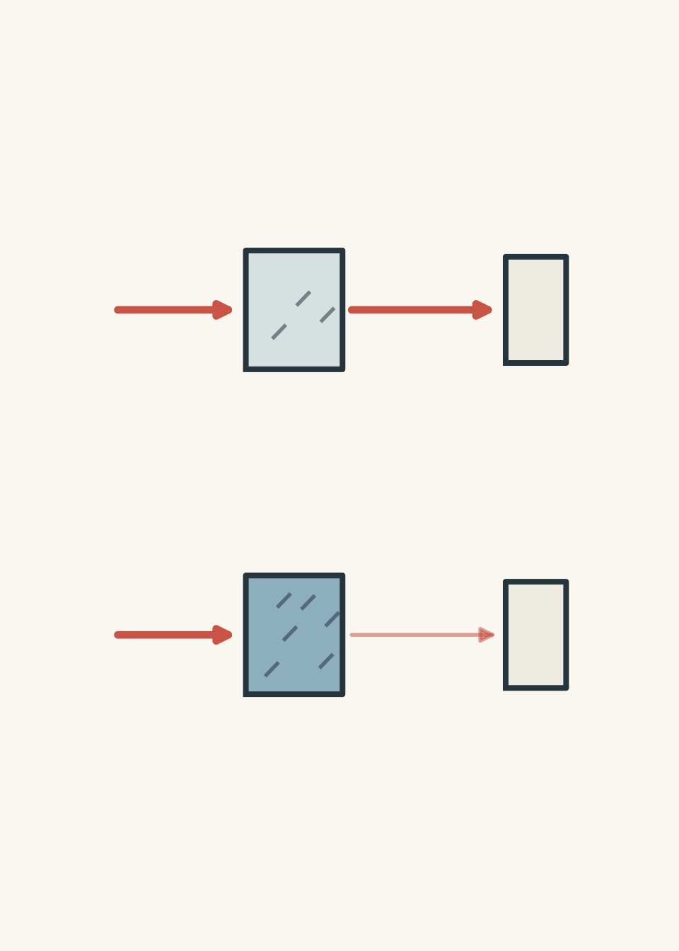
A useful first model is to imagine the absorbing particles as people standing in front of a doorway. A nearly empty doorway lets most people through. Pack the doorway with students who have just heard there are free sausage rolls outside, and fewer people make it through cleanly.
Here:
- the doorway represents the light path through the solution
- the crowd represents the absorbing particles
- the people trying to pass through represent the incoming light
The analogy has limits. Molecules do not physically block light like tiny walls. They absorb particular wavelengths of electromagnetic radiation through interactions with their electrons. But the crowd model gets the important relationship right: more absorbing particles generally means less transmitted light.
02What does a colourimeter actually measure?
A colourimeter sends light of a selected wavelength through a sample and measures how much light emerges.
Two related quantities are commonly used:
- transmittance, which describes the fraction of incident light that passes through
- absorbance, which describes how strongly the sample absorbs the light
If \(I_0\) is the intensity of light entering the sample and \(I\) is the intensity leaving it, the transmittance \(T\) is
\[ T = \frac{I}{I_0} \]
Absorbance \(A\) is related to transmittance by
\[ A = -\log_{10}(T) \]
So if half the light passes through, \(T = 0.50\), and
\[ A = -\log_{10}(0.50) = 0.301 \]
A higher absorbance means the solution has absorbed a greater fraction of the selected light.
Why not just use percentage transmittance?
Because absorbance has a particularly useful relationship with concentration.
Under suitable conditions, the Beer-Lambert relationship is
\[ A = \varepsilon lc \]
where:
- \(A\) is absorbance and has no unit
- \(\varepsilon\) is the molar absorptivity, usually in \(\mathrm{L\,mol^{-1}\,cm^{-1}}\)
- \(l\) is the path length through the solution, usually in \(\mathrm{cm}\)
- \(c\) is the concentration, usually in \(\mathrm{mol\,L^{-1}}\)
For a fixed substance, wavelength, and cuvette, \(\varepsilon\) and \(l\) remain constant. That means
\[ A \propto c \]
So, within the useful range of the method, doubling concentration should approximately double absorbance.
That linear relationship is what makes colourimetry useful for quantitative analysis.
03Why use a calibration curve?
You might be tempted to measure an unknown sample once and put its absorbance directly into \(A = \varepsilon lc\).
Sometimes that is possible. In HSC-style experimental analysis, however, you will often determine concentration using a set of known standards.
Suppose you prepare several copper(II) solutions of known concentration and measure their absorbance:
| Concentration (\(\mathrm{mol\,L^{-1}}\)) | Absorbance |
|---|---|
| 0.020 | 0.12 |
| 0.040 | 0.24 |
| 0.060 | 0.36 |
| 0.080 | 0.48 |
| 0.100 | 0.60 |
Plot absorbance on the vertical axis against concentration on the horizontal axis.
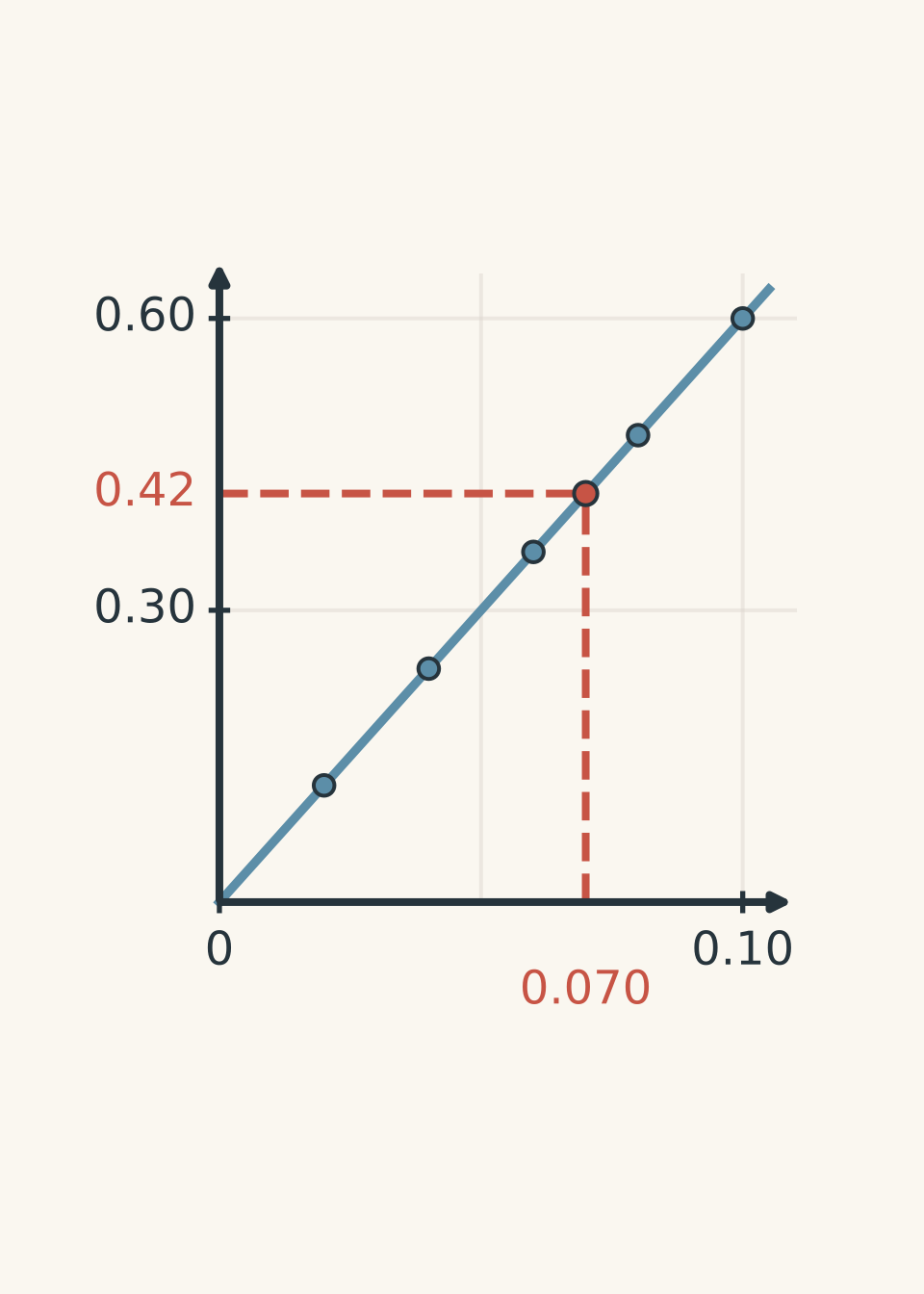
The gradient is
\[ \frac{0.60-0.12}{0.100-0.020} = 6.0\ \mathrm{L\,mol^{-1}} \]
so the calibration relationship is
\[ A = 6.0c \]
An unknown solution with absorbance \(0.42\) therefore has concentration
\[ c = \frac{A}{6.0} = \frac{0.42}{6.0} = 0.070\ \mathrm{mol\,L^{-1}} \]
The important idea is not merely “read the graph”. The standards establish how this particular measurement system responds to known concentrations. The unknown is then compared with that experimentally established relationship.
04Choosing the right wavelength
Suppose your solution appears blue. Which light should you shine through it: blue light or orange-red light?
A common first guess is blue, because the solution is blue. But that reverses what the colour tells you.
A solution appears blue because blue wavelengths are transmitted towards your eyes more strongly than the wavelengths it absorbs. To make concentration differences easier to detect, the colourimeter should use a wavelength that the species absorbs strongly.
For a blue solution, that will often be light in the complementary orange-red region.
This improves sensitivity. A small change in concentration then produces a larger measurable change in absorbance.
The exact best wavelength depends on the absorption spectrum of the species, so “always use the complementary colour” is a useful approximation rather than a universal rule. More precisely, the wavelength should usually be chosen near an absorption maximum, where absorbance is high and changes strongly with concentration.
05The blank: measuring the solute, not the container
A colourimeter does not know which absorption came from the chemical you care about.
The cuvette may absorb or scatter some light. The solvent may absorb some. Other reagents may contribute too.
A blank contains everything except the analyte being measured. The instrument is adjusted using the blank so that these background effects are accounted for.
For example, if your coloured analyte is dissolved in water and no other absorbing reagent is present, the blank may simply contain the same water in the same type of cuvette.
This is why “use an empty colourimeter” is not an adequate blank procedure. You want to subtract the optical effects of the sample environment, not remove the sample environment altogether.
06Worked example: Find an unknown concentration from a calibration equation
A student obtains the calibration relationship
\[ A = 4.80c + 0.010 \]
where \(A\) is absorbance and \(c\) is concentration in \(\mathrm{mol\,L^{-1}}\). An unknown solution gives an absorbance of \(0.394\). Determine its concentration.
Step 1
The measured absorbance \(A\) is related to concentration \(c\). We know \(A = 0.394\), so substitute that value.
\[ 0.394 = 4.80c + 0.010 \]
Step 2
\[ 0.394 - 0.010 = 4.80c \]
\[ 0.384 = 4.80c \]
Step 3
\[ c = \frac{0.384}{4.80} = 0.0800\ \mathrm{mol\,L^{-1}} \]
The unknown concentration is therefore
\[ \boxed{c = 8.00\times10^{-2}\ \mathrm{mol\,L^{-1}}} \]
The small non-zero intercept means the experimental calibration did not pass exactly through the origin. That could arise from instrumental background, imperfect blanking, or ordinary experimental uncertainty. You should use the measured calibration relationship rather than silently forcing the line through zero.
07Dilution matters
Colourimetry often gives you the concentration of the solution actually placed in the cuvette. That may not be the concentration of the original sample.
Suppose an environmental water sample is too concentrated to fit the calibration range. You dilute it, measure the diluted solution, then forget to undo the dilution.
Your colourimetry calculation could be flawless and your final answer could still be wrong.
For dilution,
\[ c_1V_1 = c_2V_2 \]
where:
- \(c_1\) is the original concentration
- \(V_1\) is the volume taken from the original solution
- \(c_2\) is the diluted concentration
- \(V_2\) is the final diluted volume
Worked example: Determine the concentration before dilution
A 10.0 mL sample is diluted to 50.0 mL. The diluted solution has absorbance \(0.328\). Its calibration relationship is
\[ A = 3.20c + 0.008 \]
where \(c\) is in \(\mathrm{mmol\,L^{-1}}\). Determine the concentration of the original sample.
Step 1
\[ 0.328 = 3.20c + 0.008 \]
\[ 0.320 = 3.20c \]
\[ c = 0.100\ \mathrm{mmol\,L^{-1}} \]
So the solution in the colourimeter contained \(0.100\ \mathrm{mmol\,L^{-1}}\).
Step 2
Using
\[ c_1V_1 = c_2V_2 \]
\[ c_1(10.0\ \mathrm{mL}) = (0.100\ \mathrm{mmol\,L^{-1}})(50.0\ \mathrm{mL}) \]
\[ c_1 = 0.500\ \mathrm{mmol\,L^{-1}} \]
The original sample concentration was therefore
\[ \boxed{0.500\ \mathrm{mmol\,L^{-1}}} \]
The fivefold dilution produced a concentration five times smaller than the original. The final answer must therefore be five times the concentration measured in the diluted sample.
08Interpolation is safer than extrapolation
Suppose your standards cover concentrations from \(0.020\) to \(0.100\ \mathrm{mol\,L^{-1}}\), but your unknown gives an absorbance that corresponds to \(0.160\ \mathrm{mol\,L^{-1}}\).
Can you just extend the line?
Mathematically, yes. Experimentally, that is risky.
Using a calibration relationship between measured standards is interpolation. Using it beyond the measured range is extrapolation.
The problem is that the linear relationship may stop being reliable at higher concentrations. Instrument response can also become less reliable when very little light reaches the detector.
A better procedure is usually to dilute the unknown until its absorbance lies within the calibration range, measure it again, then account for the dilution.
This same habit matters in broader chemical monitoring: a numerical result is only useful if the method used to obtain it is valid. That becomes especially important when analytical results are used to make environmental decisions, as discussed in Environmental Chemical Monitoring: From Results to Decisions.
09When the calibration graph does not behave
A perfect textbook calibration graph is straight. Real data may not be.
Consider these results:
| Concentration (\(\mathrm{mg\,L^{-1}}\)) | Absorbance |
|---|---|
| 2.0 | 0.11 |
| 4.0 | 0.22 |
| 6.0 | 0.33 |
| 8.0 | 0.44 |
| 10.0 | 0.46 |
The first four points show a clear linear trend. The fifth point does not.
A weak response would be: “The 10.0 mg L\(^{-1}\) result is wrong.”
That is too confident. The data show that it is inconsistent with the trend. They do not, by themselves, prove why.
Possible explanations include:
- incorrect preparation of that standard
- contamination
- fingerprints or droplets on the cuvette
- inconsistent cuvette orientation
- bubbles in the light path
- instrumental limitations
- departure from linear behaviour at higher concentration
The next experimental move should depend on the suspected cause. Repeating the measurement can help distinguish a random reading problem from a reproducible effect. Preparing a fresh standard can test whether the solution itself was prepared incorrectly.
10The most tempting misconception: darker means linearly more concentrated
If one solution looks twice as dark as another, is it twice as concentrated?
Not necessarily.
Human visual perception is not a quantitative absorbance scale. Even with an instrument, the simple linear relationship applies only under appropriate experimental conditions.
The safe reasoning is:
- colour tells you that absorption is occurring
- the colourimeter converts transmitted light into a measurement
- standards establish the relationship between absorbance and concentration
- the unknown should ideally fall within the calibrated linear range
So “darker means more concentrated” can be useful qualitatively. “Twice as dark means twice the concentration” is not a valid measurement rule.
11Evaluating colourimetry data
HSC questions often move beyond calculating a concentration. You may need to judge whether the result is trustworthy.
A useful way to analyse a colourimetry experiment is to separate four ideas:
| Question | What to inspect |
|---|---|
| Is the relationship suitable? | Do the standards show an approximately linear calibration over the range used? |
| Is the unknown inside that range? | Prefer interpolation rather than extrapolation |
| Were variables controlled? | Same wavelength, cuvette path length, solvent conditions, and measurement procedure |
| Is the result reproducible? | Repeated readings should be reasonably consistent |
Accuracy and precision are also different.
Precision is about how closely repeated measurements agree with each other.
Accuracy is about how close a result is to the accepted or true value.
A set of absorbances could be tightly grouped and therefore precise while all being shifted by the same systematic error. For example, a badly prepared blank could affect every reading in the same direction.
That means repeating a measurement does not automatically remove systematic error.
12What happens if the cuvette changes?
The Beer-Lambert relationship contains path length:
\[ A = \varepsilon lc \]
So suppose the concentration stays exactly the same but the light travels through twice the distance in the solution.
What should happen?
If the Beer-Lambert relationship applies, absorbance doubles because \(l\) doubles.
That is why standards and unknowns should be measured using the same cuvette geometry. A calibration curve does not depend only on “the chemical”. It depends on the measurement conditions used to produce it.
13Questions and solutions
Question 1
A calibration relationship for a coloured ion is
\[ A = 5.00c \]
where \(c\) is in \(\mathrm{mol\,L^{-1}}\). An unknown solution has absorbance \(0.350\).
Calculate its concentration.
Solution 1
The concentration is \(0.0700\ \mathrm{mol\,L^{-1}}\).
The calibration relationship directly connects absorbance and concentration:
\[ A = 5.00c \]
Substitute \(A = 0.350\):
\[ 0.350 = 5.00c \]
\[ c = \frac{0.350}{5.00} = 0.0700\ \mathrm{mol\,L^{-1}} \]
Therefore,
\[ \boxed{c = 7.00\times10^{-2}\ \mathrm{mol\,L^{-1}}} \]
The common mistake is to multiply \(0.350\) by \(5.00\). The gradient tells us how much absorbance is produced per unit concentration, so concentration is found by dividing absorbance by the gradient.
Question 2
A student prepares the following calibration standards.
| Concentration (\(\mathrm{mg\,L^{-1}}\)) | Absorbance |
|---|---|
| 1.0 | 0.080 |
| 2.0 | 0.159 |
| 3.0 | 0.241 |
| 4.0 | 0.320 |
An unknown gives an absorbance of \(0.280\).
Estimate its concentration and explain why this estimate is more reliable than using the same calibration line for an unknown with absorbance \(0.700\).
Solution 2
The first unknown has a concentration of approximately \(3.5\ \mathrm{mg\,L^{-1}}\), and this estimate is more reliable because it is obtained by interpolation within the calibrated range.
The data are very close to the relationship
\[ A \approx 0.080c \]
where \(c\) is in \(\mathrm{mg\,L^{-1}}\).
For \(A = 0.280\):
\[ c = \frac{0.280}{0.080} = 3.5\ \mathrm{mg\,L^{-1}} \]
So,
\[ \boxed{c \approx 3.5\ \mathrm{mg\,L^{-1}}} \]
This value lies between the standards at \(3.0\) and \(4.0\ \mathrm{mg\,L^{-1}}\), so it is an interpolation.
An absorbance of \(0.700\) would correspond to
\[ c = \frac{0.700}{0.080} = 8.75\ \mathrm{mg\,L^{-1}} \]
but the calibration data only extend to \(4.0\ \mathrm{mg\,L^{-1}}\). Using the line at \(8.75\ \mathrm{mg\,L^{-1}}\) would therefore be extrapolation.
The tempting route is to say that both calculations use the same equation, so both are equally valid. The problem is experimental, not algebraic: the standards only demonstrate linear behaviour over the measured range. The unknown with absorbance \(0.700\) should preferably be diluted and remeasured within that range.
Question 3
A 5.00 mL sample of an unknown solution is diluted to 25.00 mL. The diluted solution gives an absorbance of \(0.410\).
The calibration relationship is
\[ A = 2.00c + 0.010 \]
where \(c\) is in \(\mathrm{mmol\,L^{-1}}\).
Calculate the concentration of the original solution.
Solution 3
The original concentration is \(1.00\ \mathrm{mmol\,L^{-1}}\).
First find the concentration of the diluted solution:
\[ 0.410 = 2.00c + 0.010 \]
\[ 0.400 = 2.00c \]
\[ c = 0.200\ \mathrm{mmol\,L^{-1}} \]
Now use the dilution relationship
\[ c_1V_1 = c_2V_2 \]
with:
- \(c_1\) = original concentration
- \(V_1 = 5.00\ \mathrm{mL}\)
- \(c_2 = 0.200\ \mathrm{mmol\,L^{-1}}\)
- \(V_2 = 25.00\ \mathrm{mL}\)
\[ c_1(5.00) = (0.200)(25.00) \]
\[ c_1 = 1.00\ \mathrm{mmol\,L^{-1}} \]
Therefore,
\[ \boxed{c_1 = 1.00\ \mathrm{mmol\,L^{-1}}} \]
The tempting mistake is to report \(0.200\ \mathrm{mmol\,L^{-1}}\). That is only the concentration after dilution. Since the original 5.00 mL was diluted to 25.00 mL, its concentration was reduced by a factor of five.
Question 4
A student prepares five standards of the same coloured complex and measures each one once.
| Concentration (\(\mathrm{\mu mol\,L^{-1}}\)) | Absorbance |
|---|---|
| 10 | 0.102 |
| 20 | 0.201 |
| 30 | 0.301 |
| 40 | 0.399 |
| 50 | 0.356 |
The student says:
“The 50 \(\mathrm{\mu mol\,L^{-1}}\) point must be an outlier, so I will delete it and use the first four points.”
Evaluate that decision and describe a stronger experimental response.
Solution 4
The student should not automatically delete the 50 \(\mathrm{\mu mol\,L^{-1}}\) result. It is clearly inconsistent with the trend, but one measurement is not enough to establish the cause.
The first four standards show approximately
\[ A \approx 0.0100c \]
where \(c\) is in \(\mathrm{\mu mol\,L^{-1}}\). If that relationship continued, the expected absorbance at \(50\ \mathrm{\mu mol\,L^{-1}}\) would be about
\[ A \approx (0.0100)(50) = 0.500 \]
The measured value, \(0.356\), is therefore much lower than expected.
It is reasonable to suspect a problem, but several explanations remain possible. The 50 \(\mathrm{\mu mol\,L^{-1}}\) solution may have been prepared incorrectly, the cuvette could have contained a bubble or contamination, the instrument could have produced a faulty reading, or the system might genuinely be departing from linear behaviour.
A stronger response would be to repeat the measurement and, ideally, prepare a fresh 50 \(\mathrm{\mu mol\,L^{-1}}\) standard. Additional standards around the upper part of the range could also test whether the calibration begins to curve.
The tempting route is to treat “does not fit the line” as equivalent to “bad data”. That assumes the straight-line model is already known to be correct at \(50\ \mathrm{\mu mol\,L^{-1}}\). But the calibration experiment is partly testing that very assumption.
If repeated, correctly prepared high-concentration standards continued to fall below the linear prediction, then the appropriate conclusion would be that the linear calibration range ends before that concentration.
Question 5
A laboratory uses standards from \(0\) to \(8.0\ \mathrm{mg\,L^{-1}}\), producing a straight calibration line
\[ A = 0.100c \]
where \(c\) is in \(\mathrm{mg\,L^{-1}}\).
An unknown sample initially gives \(A = 1.20\). Because this is above the calibration range, a student dilutes 10.0 mL of the unknown to 20.0 mL.
The diluted sample gives \(A = 0.58\).
Another student argues:
“The first reading predicts \(12.0\ \mathrm{mg\,L^{-1}}\). After a twofold dilution, the absorbance should be exactly \(0.60\). We measured \(0.58\), so the dilution must have been inaccurate.”
Is that conclusion justified? Determine the best concentration estimate supported by the experiment and explain the reasoning.
Solution 5
No. The conclusion is not justified. The strongest estimate is \(11.6\ \mathrm{mg\,L^{-1}}\) for the original sample, based on the diluted measurement, and the difference between \(0.60\) and \(0.58\) does not by itself prove that the dilution was inaccurate.
The original absorbance was \(1.20\). If the calibration equation were extended beyond its established range,
\[ 1.20 = 0.100c \]
would give
\[ c = 12.0\ \mathrm{mg\,L^{-1}} \]
However, the standards only extend to \(8.0\ \mathrm{mg\,L^{-1}}\), corresponding to a maximum calibrated absorbance of
\[ A = (0.100)(8.0) = 0.80 \]
So the original reading of \(1.20\) lies outside the demonstrated calibration range. The value \(12.0\ \mathrm{mg\,L^{-1}}\) is an extrapolation, not a securely measured concentration.
Now use the diluted reading, which lies inside the calibration range:
\[ 0.58 = 0.100c_{\text{diluted}} \]
\[ c_{\text{diluted}} = 5.8\ \mathrm{mg\,L^{-1}} \]
The sample was diluted from 10.0 mL to 20.0 mL, so the dilution factor was
\[ \frac{20.0}{10.0}=2.00 \]
Therefore,
\[ c_{\text{original}} = (5.8\ \mathrm{mg\,L^{-1}})(2.00) = 11.6\ \mathrm{mg\,L^{-1}} \]
Thus,
\[ \boxed{c_{\text{original}} = 11.6\ \mathrm{mg\,L^{-1}}} \]
The subtle trap is to treat the extrapolated \(12.0\ \mathrm{mg\,L^{-1}}\) value as the benchmark and then judge the diluted result against it. That reverses the evidential strength of the two measurements.
The \(0.58\) reading was obtained inside the established calibration range, so it is the stronger evidence. The original \(1.20\) reading tells us that the sample was too concentrated for the existing calibration, but it does not establish that its concentration was exactly \(12.0\ \mathrm{mg\,L^{-1}}\).
If the linear relationship happened to remain exact beyond the calibrated range, a perfect twofold dilution would indeed give \(A = 0.60\). But the experiment has not established that assumption. The difference between \(0.60\) and \(0.58\) could arise from ordinary measurement uncertainty, dilution uncertainty, or non-linearity in the original high-absorbance region.
The key principle is that a calculation can be mathematically neat while resting on an experimentally unsupported assumption.
14Where colourimetry leads next
Colourimetry gives you a general analytical pattern that appears throughout HSC Chemistry:
known standards → measured signal → calibration relationship → unknown concentration → evaluation of reliability
The instrument may change, but the reasoning survives. You need to know what is being measured, whether the calibration applies to the unknown, and whether sample preparation has changed the concentration before measurement.
That same distinction between a measured signal and the chemical quantity you actually want is useful when studying other quantitative methods. For example, Precipitation Titrations: Calculate an Unknown Concentration uses a completely different experimental signal, but the central job is similar: connect an observation to stoichiometry or calibration carefully enough that the final concentration means what you think it means.