
Environmental Chemical Monitoring: From Results to Decisions
A lower concentration does not always mean less pollution. Learn how sampling, chemical form, and water flow affect environmental decisions through worked examples and five practice questions with full solutions.
After heavy rain, a creek’s dissolved copper concentration falls by half. Has the pollution problem improved? Make a prediction before reading on.
Not necessarily. There may be less copper entering the creek, but there may simply be more water diluting it. The creek could even be carrying more copper downstream each hour while containing less copper per litre.
Environmental chemical monitoring helps distinguish those explanations. The goal is not just to produce a concentration. It is to produce evidence that supports a particular decision.
01Why measure chemicals repeatedly?
Imagine adding water to a jug of cordial. Each sip becomes weaker, but the amount of cordial in the jug has not decreased. The cordial represents the chemical being monitored, while its strength represents concentration.
That model explains dilution. A creek adds complications: water keeps moving, inputs change, and chemicals can move between the water and sediment. Monitoring has to account for those changes, rather than treating the creek as one permanently mixed jug.
The mere presence of a chemical does not establish a pollution problem. Copper, for example, occurs naturally, and small amounts are needed by organisms. Excessive exposure can be toxic. Some metals can also accumulate in organisms when uptake exceeds elimination, so a water sample does not reveal every consequence of past exposure. US EPA
Environmental chemical monitoring is the planned collection and analysis of samples to investigate environmental conditions and changes. Its purpose determines what evidence is needed. Water Quality
| Decision | Evidence that helps |
|---|---|
| Investigate a possible new source | Results upstream, at the suspected discharge, and downstream, compared with earlier conditions |
| Reduce harmful exposure | Appropriate concentration measurements, including periods when exposure may peak |
| Evaluate a treatment or clean-up | Comparable measurements before and after intervention, including relevant chemical inputs and outputs |
| Decide whether further investigation is needed | Chemical results considered alongside toxicity tests or observations of affected organisms |
These are different questions. A measurement suitable for one may not settle another. Australian water-quality guidance therefore recommends combining relevant lines of evidence, rather than treating one chemical result as a complete environmental assessment. Water Quality
02Make the sample represent the question
Choose the place and time before choosing the instrument
Suppose a workshop discharges water into a creek. A downstream result alone cannot tell you how much copper was already present upstream.
An upstream control helps identify the workshop’s possible contribution. Earlier measurements provide a baseline: the conditions against which later results are compared. Neither is automatically “clean”; the point is to establish a meaningful comparison. Department of Environment Queensland
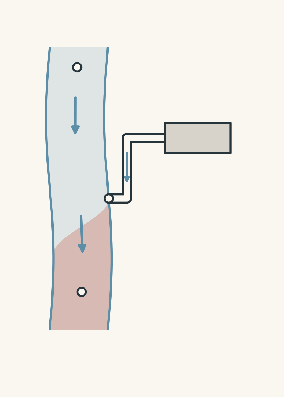
Timing matters too. Routine dry-weather sampling may miss a short runoff event. Event monitoring samples changing conditions during events such as rainfall, rather than assuming a convenient sampling time represents the whole period. Department of Environment Queensland
For our workshop investigation, a useful design would compare upstream and downstream conditions during the same discharge event, allowing for water’s travel time. Sampling should also establish whether the downstream water is sufficiently mixed for the intended comparison.
Repeatedly analysing one bottle cannot repair a poor choice of sampling location or time.
State which chemical fraction you are measuring
Copper can be dissolved in water or associated with suspended particles. These are not interchangeable measurements.
A dissolved-metals sample is operationally defined by filtration, commonly through a \(0.45\,\mu\mathrm{m}\) membrane. Here, \(\mu\mathrm{m}\) means micrometre, one millionth of a metre. “Dissolved” describes the fraction passing that filter; it does not mean that every copper-containing species is a free \(\mathrm{Cu}^{2+}\) ion. Department of Environment Queensland
An unfiltered sample can also be analysed after suitable preparation to recover copper associated with suspended solids. However, a water sample does not automatically include copper stored in the creek bed. Sediment requires its own sampling. US EPA
For the exercises below, total copper means dissolved copper plus particle-associated copper, measured by a method specified to recover both completely.
Check the measurement, not just the display
A result with several decimal places can still be wrong.
| Quality-control check | What it investigates |
|---|---|
| Blank: an analyte-free sample taken through the relevant procedure | Contamination introduced by containers, equipment, transport, or analysis |
| Duplicate samples or analyses | Repeatability: whether comparable measurements agree |
| Reference material with an independently known concentration | Whether the method gives the expected result |
The analyte is the substance being measured. These checks investigate different problems: closely agreeing duplicates demonstrate precision, but they do not prove accuracy. Both can be affected by the same systematic error. Department of Environment Queensland
Other ingredients in a sample-its matrix-may also affect the analytical response. Adding a known amount of analyte to a sample can help investigate that effect. A method must be suitable for the actual sample, not merely work well with clean laboratory standards. Department of Environment Queensland
03Turn the laboratory signal into a concentration
A qualitative analysis identifies what is present. A quantitative analysis determines how much is present.
For environmental water samples, mass concentration is often useful:
\[ c=\frac{m}{V} \]
Here, \(c\) is mass concentration in milligrams per litre, \(\mathrm{mg\,L^{-1}}\); \(m\) is analyte mass in milligrams, \(\mathrm{mg}\); and \(V\) is solution volume in litres, \(\mathrm{L}\). This is different from molar concentration, which uses moles per litre.
An instrument usually measures a signal related to concentration, rather than directly displaying the mass of copper in the creek. In atomic absorption spectroscopy, copper atoms absorb light at a characteristic wavelength. Standards with known concentrations establish the relationship between absorbance and concentration: the calibration. Agilent Technologies
All numerical monitoring data and action levels below are fictional teaching examples, not NSW environmental limits.
Worked example: Does the original sample exceed the action level?
A laboratory dilutes \(20.0\,\mathrm{mL}\) of a filtered creek sample to a final volume of \(100.0\,\mathrm{mL}\). Its validated calibration is \(A=(2.00\,\mathrm{L\,mg^{-1}})c+0.010\), where \(A\) is absorbance, which has no units, and \(c\) is copper concentration in the analysed solution.
The diluted sample has an absorbance of \(0.082\). The monitoring programme requires investigation when the original dissolved copper concentration exceeds \(0.150\,\mathrm{mg\,L^{-1}}\). Determine the original concentration and the required decision.
Step 1
The calibration intercept must be included. Not all the measured absorbance is the concentration-dependent part.
\[ \begin{aligned} c_{\text{diluted}} &=\frac{A-0.010}{2.00\,\mathrm{L\,mg^{-1}}}\\ &=\frac{0.082-0.010}{2.00\,\mathrm{L\,mg^{-1}}}\\ &=0.0360\,\mathrm{mg\,L^{-1}} \end{aligned} \]
Step 2
Dilution increases volume without changing the copper mass in the portion transferred. The final volume is five times the original sample volume, so its concentration is five times lower.
\[ \begin{aligned} c_{\text{original}} &=c_{\text{diluted}}\times\frac{\text{final volume}}{\text{sample volume}}\\ &=0.0360\,\mathrm{mg\,L^{-1}} \times\frac{100.0\,\mathrm{mL}}{20.0\,\mathrm{mL}}\\ &=0.180\,\mathrm{mg\,L^{-1}} \end{aligned} \]
The millilitre units cancel in the volume ratio.
Step 3
The original concentration, \(0.180\,\mathrm{mg\,L^{-1}}\), exceeds \(0.150\,\mathrm{mg\,L^{-1}}\). Investigation is required.
Comparing the diluted concentration directly with the action level would produce the wrong decision. The instrument analysed a laboratory preparation, not the original creek water.
04A concentration needs context
Compare like with like
Before using a guideline or action level, match the analyte, units, chemical fraction, intended water use, and required time basis.
A guideline for protecting freshwater organisms is not automatically a drinking-water standard. Nor is an average-concentration criterion interchangeable with a rule about short peaks. Australian default guideline values provide starting points for assessment; they are not automatically legal limits, although relevant authorities may incorporate them into regulatory requirements. Water Quality
The measured chemical form also matters. Bioavailability concerns how available a substance is for uptake and interaction with organisms. Water chemistry, including pH and dissolved organic matter, can influence metal bioavailability. Therefore, two samples with the same total copper concentration need not produce identical biological effects. Water Quality
“Not detected” does not mean “absent”
A method’s detection limit concerns its ability to distinguish a signal from background. Its reporting limit concerns the concentration at which it can report a result with acceptable performance. These limits are not necessarily identical.
A result reported as below a limit does not establish zero concentration. Crucially, the reporting limit must be low enough for the decision being made. A method can be reliable yet insufficiently sensitive for a particular environmental benchmark. Department of Environment Queensland
A borderline result is not an exact dividing line
Suppose a laboratory reports \(0.014\,\mathrm{mg\,L^{-1}}\), with a stated uncertainty of \(\pm0.004\,\mathrm{mg\,L^{-1}}\). An action level is \(0.015\,\mathrm{mg\,L^{-1}}\).
The central result is below the action level, but the stated interval extends from \(0.010\) to \(0.018\,\mathrm{mg\,L^{-1}}\). Simply rounding the result down does not remove that uncertainty.
The appropriate response depends on the programme’s decision rule and the consequences of error. Quality-control assessment should consider measurement uncertainty, rather than interpreting every numerical difference as a definite environmental difference. Department of Environment Queensland
05Separate concentration, chemical load, and removal
Return to the creek after rain. Concentration tells us how much copper is present per litre. To determine how much passes a point each second, we also need the water flow rate.
Let \(Q\) be flow rate in litres per second, \(\mathrm{L\,s^{-1}}\), and \(R\) be copper mass flow rate in milligrams per second, \(\mathrm{mg\,s^{-1}}\). Then:
\[ R=cQ \]
The units show why this works: \((\mathrm{mg\,L^{-1}})(\mathrm{L\,s^{-1}})=\mathrm{mg\,s^{-1}}\).
If \(R\) remains constant for a time \(t\), measured in seconds, the transported mass is \(m=Rt\). When conditions change, calculate the mass for each interval and add those masses.
This concentration-plus-flow approach is used in Australian catchment monitoring to estimate pollutant loads. Reef Plan
Worked example: Did a lower concentration mean a smaller local input?
Two steady-flow surveys investigate a copper source between upstream and downstream sampling points.
| Measurement | First survey | Second survey |
|---|---|---|
| Upstream copper concentration | \(0.010\,\mathrm{mg\,L^{-1}}\) | \(0.010\,\mathrm{mg\,L^{-1}}\) |
| Downstream copper concentration | \(0.040\,\mathrm{mg\,L^{-1}}\) | \(0.030\,\mathrm{mg\,L^{-1}}\) |
| Creek flow rate | \(200\,\mathrm{L\,s^{-1}}\) | \(400\,\mathrm{L\,s^{-1}}\) |
Assume the source adds negligible water volume, so upstream and downstream flow rates are equal within each survey. There are no other sources, and no copper is stored, released, or lost between the sampling points.
Determine whether the local copper input decreased.
Step 1
\[ \begin{aligned} R_{\text{downstream, first}} &=0.040\,\mathrm{mg\,L^{-1}}\times200\,\mathrm{L\,s^{-1}} =8.0\,\mathrm{mg\,s^{-1}}\\ R_{\text{downstream, second}} &=0.030\,\mathrm{mg\,L^{-1}}\times400\,\mathrm{L\,s^{-1}} =12\,\mathrm{mg\,s^{-1}} \end{aligned} \]
The lower concentration accompanies a higher downstream transport rate.
Step 2
Some copper was already in the creek. Under the stated assumptions, the local input is the downstream rate minus the upstream rate.
\[ \begin{aligned} R_{\text{local, first}} &=(0.040-0.010)\,\mathrm{mg\,L^{-1}}\times200\,\mathrm{L\,s^{-1}} =6.0\,\mathrm{mg\,s^{-1}}\\ R_{\text{local, second}} &=(0.030-0.010)\,\mathrm{mg\,L^{-1}}\times400\,\mathrm{L\,s^{-1}} =8.0\,\mathrm{mg\,s^{-1}} \end{aligned} \]
Step 3
The local copper input increased from \(6.0\) to \(8.0\,\mathrm{mg\,s^{-1}}\), an increase of approximately \(33\%\).
The downstream concentration did fall, which is relevant to concentration-dependent exposure. However, the evidence does not show improved control of the local input. Under this model, that input became larger.
Remember what the calculation assumed
The worked example excluded storage. A real creek may retain copper in sediment or release previously stored copper. In that case, an input-output difference must also account for the changing stored mass.
Chemical treatment cannot destroy copper atoms. It can transfer them into another chemical form or separate them from the water. Whether that counts as removal depends on the system boundary: copper removed from the water but left in the creek bed has not been removed from the creek.
That is why “the dissolved concentration fell” and “the copper was removed from the environment” are different claims.
06Questions and solutions
Treat numerical data as exact for these exercises unless stated otherwise. In Question 1, treat the reported upper bound as valid.
Question 1
A laboratory reports dissolved copper as less than \(0.020\,\mathrm{mg\,L^{-1}}\). The monitoring programme’s action level is \(0.010\,\mathrm{mg\,L^{-1}}\).
A student concludes, “There is no copper, so the creek meets the action level and further monitoring is unnecessary.”
Explain the errors, and identify a suitable change to both the analytical method and the sampling plan.
Solution 1
The result establishes neither the absence of copper nor that the action level has been met. The method needs a lower reporting limit, and representative monitoring should continue.
For example, an actual concentration of \(0.015\,\mathrm{mg\,L^{-1}}\) would be below the reported upper bound but above the action level. It is fully compatible with the laboratory result.
The analytical method should have a validated reporting limit below \(0.010\,\mathrm{mg\,L^{-1}}\), with suitable performance near that level.
The sampling plan should also cover relevant locations and changing conditions, such as upstream and downstream sites during dry weather and runoff events. Even a sufficiently sensitive analysis of this bottle would not establish conditions at other times.
The tempting mistake is to treat the laboratory’s inability to report a small concentration as evidence that the environment contains none.
Question 2
Clean copper standards give the relationship \(S=(2.00\,\mathrm{L\,mg^{-1}})c\), where \(S\) is blank-corrected absorbance and \(c\) is copper concentration.
A creek sample is diluted from \(20.0\,\mathrm{mL}\) to \(100.0\,\mathrm{mL}\). Two analyses of the diluted sample both give \(S=0.0180\).
A matched portion receives an additional \(0.0200\,\mathrm{mg\,L^{-1}}\) of copper, with negligible volume change. Its absorbance is \(0.0380\).
Assume the sample matrix changes the sensitivity by a constant factor, affects the original and added copper equally, and produces no additional absorbance. The response remains linear.
The action level for the original sample is \(0.0750\,\mathrm{mg\,L^{-1}}\). Determine whether it is exceeded, and explain why the duplicate results did not reveal the problem.
Solution 2
The original concentration is \(0.0900\,\mathrm{mg\,L^{-1}}\), so it exceeds the action level. The duplicates agree because the same matrix effect affects both measurements.
Step 1: Use the known addition to determine the sensitivity in this sample.
The added copper increases absorbance by \(0.0380-0.0180=0.0200\). Therefore:
\[ \begin{aligned} \text{sample sensitivity} &=\frac{\text{increase in absorbance}}{\text{added concentration}}\\ &=\frac{0.0200}{0.0200\,\mathrm{mg\,L^{-1}}}\\ &=1.00\,\mathrm{L\,mg^{-1}} \end{aligned} \]
This is half the sensitivity obtained with clean standards.
Step 2: Calculate the original concentration using that sensitivity.
\[ \begin{aligned} c_{\text{diluted}} &=\frac{0.0180}{1.00\,\mathrm{L\,mg^{-1}}} =0.0180\,\mathrm{mg\,L^{-1}}\\ c_{\text{original}} &=0.0180\,\mathrm{mg\,L^{-1}}\times\frac{100.0}{20.0}\\ &=0.0900\,\mathrm{mg\,L^{-1}} \end{aligned} \]
Step 3: Explain the misleading result.
Using the clean-standard sensitivity would instead give:
\[ c_{\text{incorrect}} =\frac{0.0180}{2.00\,\mathrm{L\,mg^{-1}}}\times5.00 =0.0450\,\mathrm{mg\,L^{-1}} \]
That incorrect result lies below the action level.
The duplicates show repeatability, not freedom from bias. Under the question’s assumptions, the known addition supplies the missing information: how strongly copper actually responds in this sample.
Question 3
A treatment adds base to copper-containing water but does not capture any resulting solids. Representative samples give these results:
| Measurement | Before treatment | After treatment |
|---|---|---|
| Total copper | \(0.120\,\mathrm{mg\,L^{-1}}\) | \(0.120\,\mathrm{mg\,L^{-1}}\) |
| Copper in samples filtered immediately | \(0.100\,\mathrm{mg\,L^{-1}}\) | \(0.010\,\mathrm{mg\,L^{-1}}\) |
All quality-control checks pass.
A second technician acidifies an unfiltered after-treatment sample, completely dissolving its copper-containing solids, and then filters it. The result is \(0.120\,\mathrm{mg\,L^{-1}}\).
The action level applies to dissolved copper in the receiving water and is \(0.020\,\mathrm{mg\,L^{-1}}\).
Explain whether the treatment destroyed copper, reconcile the two after-treatment filtered results, and state what decision the evidence supports. Include a possible precipitation equation and calculate the particle-associated copper concentrations.
Solution 3
The treatment did not destroy copper. It reduced the measured dissolved concentration by transferring copper into particles, while total copper remained unchanged. The immediately filtered result is below the action level at sampling; the acidified result does not contradict it.
A possible precipitation reaction is:
\[ \ce{Cu^2+(aq) + 2OH-(aq) -> Cu(OH)2(s)} \]
The copper atoms remain present in the solid. The data are consistent with this mechanism, although identifying the actual solid would require further evidence.
Particle-associated copper is the difference between total and dissolved copper:
\[ \begin{aligned} c_{\text{particles, before}} &=0.120-0.100 =0.020\,\mathrm{mg\,L^{-1}}\\ c_{\text{particles, after}} &=0.120-0.010 =0.110\,\mathrm{mg\,L^{-1}} \end{aligned} \]
The dissolved fraction lost \(0.090\,\mathrm{mg\,L^{-1}}\), while the particle-associated fraction gained the same amount.
The second technician changed the sample before separating its fractions. Acid can dissolve copper hydroxide:
\[ \ce{Cu(OH)2(s) + 2H+(aq) -> Cu^2+(aq) + 2H2O(l)} \]
Copper that was particulate in the receiving water was therefore dissolved when that technician filtered the bottle. Their result describes the acid-treated sample, not the original dissolved fraction.
The supported conclusion is limited but useful: the immediately filtered sample contains \(0.010\,\mathrm{mg\,L^{-1}}\), below the stated dissolved-copper action level. It does not establish permanent protection. The uncaptured copper-containing particles remain an issue, particularly if later conditions allow copper to return to solution.
The trap is to assume that accurate measurements must disagree whenever their numbers differ. Here, both can be accurate because they measure chemically different preparations.
Question 4
A three-hour discharge has a constant copper concentration within each hour, but the concentrations may differ between hours.
| Hour | Water flow rate |
|---|---|
| 1 | \(100\,\mathrm{L\,s^{-1}}\) |
| 2 | \(200\,\mathrm{L\,s^{-1}}\) |
| 3 | \(300\,\mathrm{L\,s^{-1}}\) |
One composite sample combines equal volumes from the three hours. Another combines volumes in proportion to the water discharged during each hour. Both composites contain \(0.020\,\mathrm{mg\,L^{-1}}\) of dissolved copper.
Assume representative sampling, non-negative concentrations, and no chemical changes or losses in either composite. An action level is exceeded if any hourly concentration is greater than \(0.035\,\mathrm{mg\,L^{-1}}\).
Determine whether the composite results rule out an exceedance. Construct both a non-exceeding and an exceeding concentration history consistent with the results, find the largest possible hourly concentration, and identify which single hourly sample would settle the exceedance question.
Solution 4
The composites do not rule out an exceedance. The largest possible hourly concentration is \(0.060\,\mathrm{mg\,L^{-1}}\), and only Hour 2 can exceed the action level. Analysing its separately retained sample would settle the question under this model.
Step 1: Translate each composite into its own constraint.
Let \(c_1\), \(c_2\), and \(c_3\) be the hourly concentrations, all in \(\mathrm{mg\,L^{-1}}\).
Equal sample volumes give equal weighting. The flow-proportional composite gives weights of \(1:2:3\), because the hours have equal duration.
\[ \begin{aligned} \frac{c_1+c_2+c_3}{3} &=0.020\,\mathrm{mg\,L^{-1}}\\ \frac{c_1+2c_2+3c_3}{6} &=0.020\,\mathrm{mg\,L^{-1}} \end{aligned} \]
Multiplying through, then subtracting twice the first resulting equation from the second, gives \(c_3=c_1\). Therefore:
\[ c_2=0.060\,\mathrm{mg\,L^{-1}}-2c_1 \]
The matching composite results do not require three equal concentrations. They require the first and third concentrations to match.
Step 2: Construct two compatible histories.
A non-exceeding history is \(0.020,\ 0.020,\ 0.020\,\mathrm{mg\,L^{-1}}\).
An exceeding history is \(0.005,\ 0.050,\ 0.005\,\mathrm{mg\,L^{-1}}\). For that history:
\[ \begin{aligned} \text{equal-volume result} &=\frac{0.005+0.050+0.005}{3} =0.020\,\mathrm{mg\,L^{-1}}\\ \text{flow-proportional result} &=\frac{0.005+2(0.050)+3(0.005)}{6} =0.020\,\mathrm{mg\,L^{-1}} \end{aligned} \]
Both measured averages are reproduced, despite the Hour 2 exceedance.
Step 3: Use non-negativity to find the limits.
Because \(c_2\geq0\), the relation above requires \(c_1\leq0.030\,\mathrm{mg\,L^{-1}}\). Since \(c_3=c_1\), neither Hour 1 nor Hour 3 can exceed \(0.035\,\mathrm{mg\,L^{-1}}\).
Hour 2 reaches its maximum when \(c_1=c_3=0\). Then \(c_2=0.060\,\mathrm{mg\,L^{-1}}\).
The next measurement is therefore not an arbitrary extra sample: it is the Hour 2 sample.
The tempting conclusion is that two agreeing averages confirm steady conditions. They do not. Each compresses a time history, and different histories can produce the same compressed results.
Question 5
Two model ponds each contain \(100.0\,\mathrm{L}\) of water. They initially have the same pH and negligible dissolved copper.
One pond retains its original sediment. A clean-up removes \(90.0\%\) of both solids from the other pond:
| Solid remaining | Untreated pond | Cleaned pond |
|---|---|---|
| \(\ce{CaCO3}\) | \(1.00\,\mathrm{mmol}\) | \(0.100\,\mathrm{mmol}\) |
| \(\ce{CuO}\) | \(0.100\,\mathrm{mmol}\) | \(0.0100\,\mathrm{mmol}\) |
A millimole, \(\mathrm{mmol}\), is \(10^{-3}\) moles.
Use this idealised model: added acid reacts completely with accessible calcium carbonate before attacking copper oxide. Copper released from the oxide remains dissolved. Ignore other reactions, baseline dissolution, and volume changes.
\[ \begin{aligned} &\ce{CaCO3(s) + 2H+(aq) -> Ca^2+(aq) + CO2(g) + H2O(l)}\\ &\ce{CuO(s) + 2H+(aq) -> Cu^2+(aq) + H2O(l)} \end{aligned} \]
These reaction-order assumptions are supplied model rules, not a universal description of natural sediment. Compare dissolved copper only, not other possible environmental harms.
First, find the full range of a single storm’s acid amount, \(a\), for which the cleaned pond develops a greater dissolved copper concentration than the untreated pond.
Then consider two successive storms, each adding \(1.10\,\mathrm{mmol}\) of \(\mathrm{H}^{+}\) to each pond. Between storms, all water is replaced with fresh water, removing dissolved substances but leaving the remaining solids. Calculate dissolved copper concentrations after each storm.
Use \(63.5\,\mathrm{mg\,mmol^{-1}}\) as copper’s molar mass. Assess the claim, “A smaller remaining copper inventory guarantees a lower concentration in every future storm.”
Solution 5
The claim is false. For a single storm, the cleaned pond releases more copper when \(0.200\,\mathrm{mmol}<a<2.020\,\mathrm{mmol}\). In the two-storm sequence, the cleaned pond releases copper first, but the untreated pond releases ten times as much copper during the second storm.
The clean-up reduced the copper inventory, but it also removed material that protected that inventory from acid.
Step 1: Calculate each pond’s initial acid-neutralising capacity.
Each mole of calcium carbonate consumes two moles of hydrogen ions.
\[ \begin{aligned} \text{untreated carbonate capacity} &=2(1.00\,\mathrm{mmol}) =2.00\,\mathrm{mmol\ of\ }\mathrm{H}^{+}\\ \text{cleaned carbonate capacity} &=2(0.100\,\mathrm{mmol}) =0.200\,\mathrm{mmol\ of\ }\mathrm{H}^{+} \end{aligned} \]
Copper release begins only after the relevant carbonate capacity is exhausted.
Step 2: Find where the single-storm ranking changes.
For \(a\leq0.200\,\mathrm{mmol}\), neither pond releases copper.
Above \(0.200\,\mathrm{mmol}\), the cleaned pond begins releasing copper while the untreated pond remains protected. However, the cleaned pond can release no more than its entire \(0.0100\,\mathrm{mmol}\) copper inventory.
The untreated pond catches up with that amount after consuming its carbonate and then enough acid to dissolve \(0.0100\,\mathrm{mmol}\) of copper oxide:
\[ \begin{aligned} a_{\text{catch-up}} &=2.00\,\mathrm{mmol}+2(0.0100\,\mathrm{mmol})\\ &=2.020\,\mathrm{mmol} \end{aligned} \]
Thus, the cleaned pond has the greater dissolved concentration for:
\[ 0.200\,\mathrm{mmol}<a<2.020\,\mathrm{mmol} \]
At the upper boundary, the concentrations are equal. Above it, the untreated pond releases more copper.
Two constraints determine the reversal: carbonate consumes acid before copper is released, and copper release cannot exceed the remaining copper inventory.
Step 3: Track the first storm.
In the untreated pond, \(1.10\,\mathrm{mmol}\) of hydrogen ions consumes:
\[ n_{\ce{CaCO3}\text{ consumed}} =\frac{1.10\,\mathrm{mmol}}{2} =0.550\,\mathrm{mmol} \]
Here, \(n\) denotes amount of substance. The pond retains \(1.00-0.550=0.450\,\mathrm{mmol}\) of calcium carbonate. No copper oxide reacts, so dissolved copper remains zero in this model.
The cleaned pond uses \(0.200\,\mathrm{mmol}\) of acid on carbonate. Its remaining \(0.900\,\mathrm{mmol}\) of acid is more than enough to dissolve all \(0.0100\,\mathrm{mmol}\) of copper oxide, which requires only \(0.0200\,\mathrm{mmol}\).
\[ \begin{aligned} m_{\ce{Cu}} &=0.0100\,\mathrm{mmol}\times63.5\,\mathrm{mg\,mmol^{-1}} =0.635\,\mathrm{mg}\\ c_{\text{cleaned, storm 1}} &=\frac{0.635\,\mathrm{mg}}{100.0\,\mathrm{L}} =0.00635\,\mathrm{mg\,L^{-1}} \end{aligned} \]
Step 4: Replace the water, but do not reset the sediment.
The untreated pond still has \(0.450\,\mathrm{mmol}\) of calcium carbonate. During the second storm, it consumes \(0.900\,\mathrm{mmol}\) of hydrogen ions.
The acid remaining for copper oxide is:
\[ \begin{aligned} n_{\mathrm{H}^{+}\text{ remaining}} &=1.10-0.900 =0.200\,\mathrm{mmol}\\ n_{\ce{Cu}\text{ released}} &=\frac{0.200\,\mathrm{mmol}}{2} =0.100\,\mathrm{mmol}\\ c_{\text{untreated, storm 2}} &=\frac{0.100\,\mathrm{mmol}\times63.5\,\mathrm{mg\,mmol^{-1}}} {100.0\,\mathrm{L}}\\ &=0.0635\,\mathrm{mg\,L^{-1}} \end{aligned} \]
The cleaned pond has no copper oxide left, so its second-storm copper concentration is zero.
| Pond | After Storm 1 | After Storm 2 |
|---|---|---|
| Untreated | \(0\,\mathrm{mg\,L^{-1}}\) | \(0.0635\,\mathrm{mg\,L^{-1}}\) |
| Cleaned | \(0.00635\,\mathrm{mg\,L^{-1}}\) | \(0\,\mathrm{mg\,L^{-1}}\) |
Step 5: Separate earlier release from greater total release.
The cleaned pond releases less copper across both storms: \(0.635\,\mathrm{mg}\), compared with \(6.35\,\mathrm{mg}\). Nevertheless, it has the higher concentration during the first storm.
A first-storm result alone could therefore make the clean-up look as though it introduced copper. It did not. It allowed some pre-existing copper to dissolve earlier by reducing the carbonate reserve.
The matching initial pH and dissolved copper results concealed different solid inventories and different acid-neutralising capacities. Predicting future release requires those measurements, together with information about incoming acid amounts. Measuring the current water alone does not reveal how the system will respond when conditions change.
07What to decide before ordering the next test
Start with the decision: current exposure, transported mass, source contribution, or possible future release. That determines the sampling locations, timing, chemical fraction, and analytical performance you need.
Then choose the analytical technique. Equilibrium and solubility explain how a chemical can move between measured fractions; monitoring tests whether those changes are occurring. Together, they let you interpret a low concentration as evidence about particular conditions-not as a promise about the next storm.