
Atomic Absorption Spectroscopy for HSC Chemistry
Learn how atomic absorption spectroscopy measures metal concentrations in aqueous samples using atomisation, selective absorption, calibration curves, and dilution calculations.
Suppose a river sample contains copper ions, but the solution looks completely clear. You still need to decide whether the copper concentration is low enough to be acceptable, and a colour change won’t rescue you.
So how can an instrument measure a metal ion that you cannot see?
Imagine sending one very specific colour of light through a cloud of copper atoms. If the atoms are able to absorb that exact light, less of it reaches the detector. Now make the sample more concentrated. There are more copper atoms in the light path, so more light is absorbed.
That is the central idea behind atomic absorption spectroscopy, or AAS.
Before going further, predict this: if you shine the same wavelength of light through equal volumes of a dilute copper solution and a concentrated copper solution, which should absorb more?
The concentrated sample should absorb more. That sounds simple, but AAS needs several extra steps before that idea becomes a reliable concentration measurement.
01What AAS is actually measuring
AAS is commonly used to determine the concentration of metal ions in aqueous samples.
A liquid sample might contain ions such as \(\mathrm{Cu}^{2+}\), \(\mathrm{Fe}^{3+}\), \(\mathrm{Pb}^{2+}\), or \(\mathrm{Ca}^{2+}\). However, the instrument does not simply shine light through those dissolved ions and read their concentration directly.
Instead, the sample is converted into free gaseous atoms.
That distinction matters.
A useful first model is to imagine a crowded school assembly. One particular student is waiting for one particular person to wave at them. Random waving from everyone else mostly gets ignored. In AAS, the atoms are similarly selective: atoms of a particular element absorb particular wavelengths of light.
The analogy breaks because atoms are not choosing anything. Their absorption comes from quantised electron energy levels.
02Why each element absorbs particular wavelengths
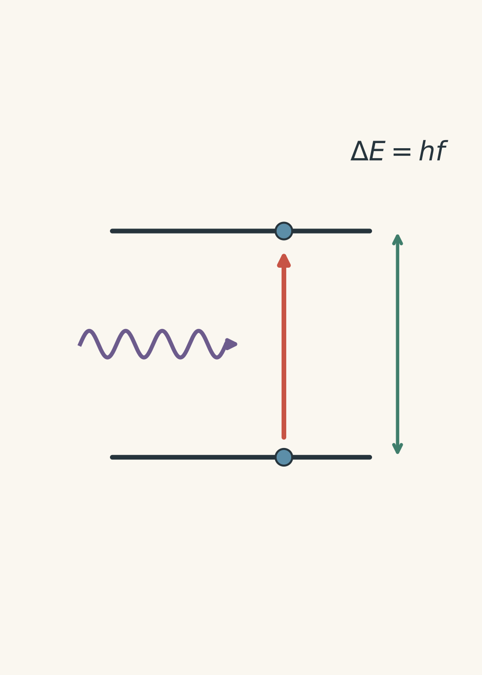
Electrons in atoms can occupy only certain energy levels.
If an atom absorbs a photon with exactly the right energy, one of its electrons can move from a lower energy level to a higher one.
The photon energy is related to its frequency by
\[ E = hf \]
where:
- \(E\) is the photon energy in joules, \(\text{J}\)
- \(h\) is Planck’s constant
- \(f\) is the frequency of the radiation in hertz, \(\text{Hz}\)
Because different elements have different allowed electron energy levels, they absorb different characteristic wavelengths.
This gives AAS its selectivity. A copper atom and a sodium atom do not have identical electron energy structures, so the instrument can choose a wavelength strongly absorbed by copper while largely ignoring sodium.
There is an important limitation to the simple picture. An element usually has several possible electronic transitions, so it can absorb several wavelengths. In practice, the instrument uses a carefully selected analytical wavelength that gives useful sensitivity with minimal interference.
03How the sample gets from a beaker to free atoms
The sample begins as an aqueous solution, but AAS needs free atoms in the gas phase.
In a common flame AAS setup, the sequence is roughly:
- The liquid sample is drawn into a nebuliser.
- The nebuliser converts the liquid into a fine aerosol.
- The aerosol enters a flame.
- Solvent evaporates.
- Dissolved substances are converted into gaseous species.
- Free atoms of the element are produced.
- Light of a selected wavelength passes through this atomic vapour.
- A detector measures how much light remains.
You should be able to mentally run the sample through the instrument in that order.
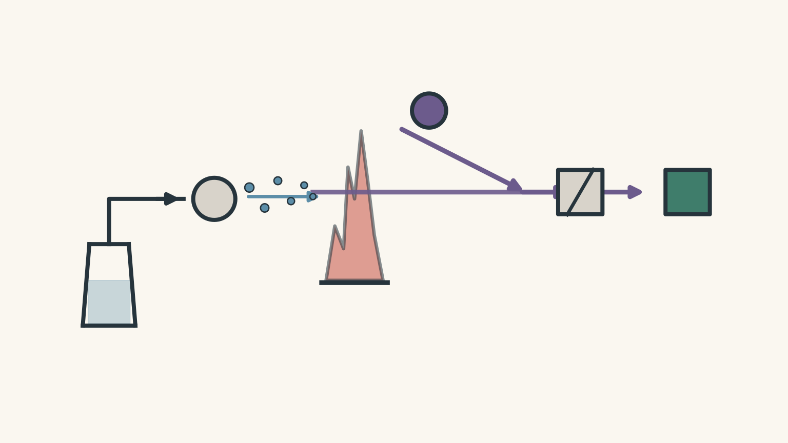
The flame is therefore doing more than “heating the sample”. Its job is to help atomise the analyte so that individual atoms can interact with the light.
04Why AAS needs an element-specific light source
Suppose you want to measure copper.
Would it make sense to shine a broad mixture of wavelengths through the flame and hope copper absorbs enough of them to identify itself?
Not very efficiently.
AAS instead uses a light source that emits wavelengths characteristic of the element being analysed. A hollow cathode lamp is commonly used for this purpose.
For a copper analysis, the lamp is chosen to provide suitable copper wavelengths. The light passes through the flame containing the atomised sample. Copper atoms absorb some of the light at the selected wavelength, so the detected intensity falls.
This is one reason AAS can be highly selective for individual metals.
05From light intensity to absorbance
The detector compares the incident light intensity with the transmitted light intensity.
Absorbance is defined by
\[ A = \log_{10}\left(\frac{I_0}{I}\right) \]
where:
- \(A\) is absorbance and has no unit
- \(I_0\) is the incident light intensity
- \(I\) is the transmitted light intensity
If very little light is absorbed, then \(I\) is close to \(I_0\), so \(A\) is small.
If more light is absorbed, \(I\) becomes smaller and \(A\) increases.
For suitable concentration ranges, greater concentration of the metal gives greater absorbance.
That is the useful relationship. But AAS usually does not turn absorbance directly into concentration from theory alone.
It uses calibration.
06Why a calibration curve is needed
Suppose an unknown sample gives an absorbance of \(0.31\).
Is that a high copper concentration? A low one?
The number means very little until the instrument response has been compared with standards of known concentration.
A set of standard solutions is prepared containing known concentrations of the metal being analysed. Their absorbances are measured under the same conditions.
For example:
| Copper concentration, \(\text{mg L}^{-1}\) | Absorbance |
|---|---|
| 0.00 | 0.002 |
| 1.00 | 0.104 |
| 2.00 | 0.207 |
| 3.00 | 0.306 |
| 4.00 | 0.410 |
The points can then be plotted as absorbance against concentration.
Over a suitable working range, the relationship is often approximately linear:
\[ A = mc + b \]
where:
- \(A\) is absorbance
- \(m\) is the gradient of the calibration line
- \(c\) is concentration
- \(b\) is the intercept
If the unknown absorbance lies within the calibrated range, its concentration can be found from the graph or calibration equation.
This is closely related to the logic used in UV-Visible spectrophotometry: known standards establish how instrument response depends on concentration, then the unknown is compared with them.
Worked example: Finding copper concentration from a calibration equation
An AAS calibration for copper gives the equation
\[ A = 0.0820c + 0.003 \]
where \(c\) is the copper concentration in \(\text{mg L}^{-1}\).
A water sample gives an absorbance of \(0.249\). Determine its copper concentration.
Step 1
\[ A = 0.0820c + 0.003 \]
Step 2
\[ 0.249 = 0.0820c + 0.003 \]
Step 3
\[ 0.249 - 0.003 = 0.0820c \]
\[ c = \frac{0.246}{0.0820} \]
\[ c = 3.00\ \text{mg L}^{-1} \]
The copper concentration in the analysed sample is \(3.00\ \text{mg L}^{-1}\).
The important point is not just the arithmetic. The unknown absorbance has been translated into concentration by comparison with known copper standards measured using the same method.
07The dilution trap
AAS samples are often diluted before measurement.
This might be done because the original sample is too concentrated for the calibration range or because sample preparation requires dilution.
The instrument then measures the diluted sample, not the original one.
A very common mistake is to calculate the concentration from the calibration curve correctly and stop there.
Consider this: a diluted sample is measured as \(2.0\ \text{mg L}^{-1}\). The original sample was diluted tenfold before analysis. Is the original concentration \(0.20\), \(2.0\), or \(20\ \text{mg L}^{-1}\)?
It is \(20\ \text{mg L}^{-1}\).
Dilution lowers concentration. Therefore, the original must have been more concentrated than the diluted sample.
For a dilution,
\[ c_1V_1 = c_2V_2 \]
where:
- \(c_1\) is the original concentration
- \(V_1\) is the original aliquot volume
- \(c_2\) is the diluted concentration
- \(V_2\) is the final diluted volume
Worked example: AAS followed by a dilution calculation
A \(10.00\ \text{mL}\) sample of wastewater is transferred to a \(100.0\ \text{mL}\) volumetric flask and diluted to the mark.
The diluted solution is analysed for zinc by AAS. Its absorbance is \(0.365\).
The calibration equation is
\[ A = 0.120c + 0.005 \]
where \(c\) is in \(\text{mg L}^{-1}\).
Determine the zinc concentration in the original wastewater.
Step 1
\[ 0.365 = 0.120c + 0.005 \]
\[ 0.360 = 0.120c \]
\[ c = 3.00\ \text{mg L}^{-1} \]
So the diluted flask contains zinc at \(3.00\ \text{mg L}^{-1}\).
Step 2
\[ c_1V_1 = c_2V_2 \]
\[ c_1(10.00\ \text{mL}) = (3.00\ \text{mg L}^{-1})(100.0\ \text{mL}) \]
\[ c_1 = 30.0\ \text{mg L}^{-1} \]
The original wastewater contained \(30.0\ \text{mg L}^{-1}\) of zinc.
Notice the direction of the answer. A tenfold dilution produced a concentration of \(3.00\ \text{mg L}^{-1}\), so the original must be ten times more concentrated.
08Why you should not extrapolate carelessly
Suppose your standards cover \(0\) to \(5.0\ \text{mg L}^{-1}\), but an unknown gives an absorbance corresponding to \(9\ \text{mg L}^{-1}\) when the calibration line is extended.
It is tempting to accept \(9\ \text{mg L}^{-1}\).
The safer method is to dilute the sample until its absorbance falls within the calibrated range, measure it again, then correct for the dilution.
Why?
Because the linear relationship between absorbance and concentration is only established over the measured calibration range. Outside that range, the instrument response may become non-linear.
Extrapolation assumes that a trend continues into a region where you have not actually tested it.
A good calibration curve is evidence. Extending the ruler beyond the last mark is an assumption.
09AAS does not measure “all metal ions at once”
One of the most tempting misconceptions is that AAS measures the overall amount of metal in a sample.
It usually does not.
AAS is selective for a particular element because the instrument uses a wavelength associated with that element.
If a sample contains copper, iron, calcium, and lead, a copper measurement does not automatically give the concentration of the other three.
Separate analytical conditions or measurements are required.
Another subtle point is that the result is normally reported as the concentration of an element, not the concentration of one particular aqueous species unless the method specifically separates species first.
For example, a measurement of total copper after suitable sample preparation may tell you the amount of copper present, but not necessarily whether that copper originally existed as free \(\mathrm{Cu}^{2+}\), a complex ion, or another dissolved form.
AAS is an elemental analysis technique.
10What makes an AAS result trustworthy?
The instrument can display many decimal places. That does not make the result automatically reliable.
Several parts of the method matter.
| Issue | Why it matters |
|---|---|
| Suitable standards | The unknown should be compared with standards covering an appropriate concentration range |
| Blank measurement | A blank helps account for absorption or signal caused by solvents, reagents, or the instrument background |
| Correct wavelength | The wavelength should be strongly and selectively absorbed by the element of interest |
| Consistent preparation | Standards and samples should be treated as similarly as practical |
| Dilution accuracy | Errors in pipetting or volumetric dilution directly affect the final concentration |
| Interferences | Other substances can change atomisation or contribute to the measured signal |
| Replicate measurements | Repeated measurements can reveal poor precision or unusual results |
A blank usually contains the solvent and relevant reagents but not the analyte being measured. Its purpose is not to create “zero chemistry”. It estimates the response that would occur even without the target analyte.
11Sensitivity, accuracy, and selectivity are different ideas
Students often blur these together.
Sensitivity describes how strongly the measured signal changes when concentration changes. On a linear calibration graph, a steeper gradient means greater sensitivity.
Accuracy describes how close the result is to the true or accepted value.
Precision describes how closely repeated measurements agree with one another.
Selectivity describes how well the method responds to the analyte of interest rather than other substances.
An instrument could produce extremely precise results that are all wrong because the calibration standard was prepared incorrectly.
That is the analytical chemistry version of repeatedly throwing darts into the wrong part of the board. Tight grouping gives precision. It does not guarantee accuracy.
The analogy breaks because analytical errors can come from several chemical and instrumental sources, not just a shifted aim.
12How AAS fits into aqueous environmental analysis
Imagine testing water downstream from an industrial site for lead.
A sensible analytical sequence might be:
- collect a representative water sample
- preserve or prepare the sample appropriately
- prepare lead standards of known concentration
- measure the standards using AAS
- construct a calibration relationship
- measure the sample
- dilute and remeasure if its signal lies outside the useful range
- calculate the original lead concentration
- consider uncertainty, interferences, blanks, and repeats
- compare the result with the relevant decision criterion
The final step matters because an analytical result is often collected to support a decision, not just to produce a number.
That broader link between chemical measurements and environmental decisions is developed further in Environmental Chemical Monitoring: From Results to Decisions.
13Questions and solutions
Question 1
A calcium standard containing \(2.00\ \text{mg L}^{-1}\) gives an absorbance of \(0.142\), while a \(4.00\ \text{mg L}^{-1}\) standard gives an absorbance of \(0.281\).
An unknown gives an absorbance of \(0.211\).
Assuming the calibration is linear in this range, estimate the calcium concentration in the unknown.
Solution 1
The calcium concentration is approximately \(3.0\ \text{mg L}^{-1}\).
The absorbance \(0.211\) lies almost halfway between \(0.142\) and \(0.281\), so the concentration should lie almost halfway between \(2.00\) and \(4.00\ \text{mg L}^{-1}\).
More precisely,
\[ \frac{0.211-0.142}{0.281-0.142} = \frac{0.069}{0.139} \approx 0.496 \]
So the concentration is
\[ c = 2.00 + 0.496(4.00-2.00) \]
\[ c \approx 2.99\ \text{mg L}^{-1} \]
Therefore,
\[ c \approx 3.0\ \text{mg L}^{-1} \]
The tempting shortcut is to assume absorbance itself equals concentration. It does not. Absorbance becomes useful only through the calibration relationship.
Question 2
A student analyses iron in a groundwater sample.
A \(5.00\ \text{mL}\) aliquot of the original sample is diluted to \(50.00\ \text{mL}\). The diluted sample gives an absorbance of \(0.428\).
The iron calibration equation is
\[ A = 0.0850c + 0.003 \]
where \(c\) is in \(\text{mg L}^{-1}\).
Calculate the iron concentration in the original groundwater.
Solution 2
The original iron concentration is \(50.0\ \text{mg L}^{-1}\).
First, use the calibration equation to find the concentration of the diluted sample:
\[ 0.428 = 0.0850c + 0.003 \]
\[ 0.425 = 0.0850c \]
\[ c = 5.00\ \text{mg L}^{-1} \]
This is not yet the original concentration.
The \(5.00\ \text{mL}\) aliquot was diluted to \(50.00\ \text{mL}\), so
\[ c_1V_1 = c_2V_2 \]
\[ c_1(5.00\ \text{mL}) = (5.00\ \text{mg L}^{-1})(50.00\ \text{mL}) \]
\[ c_1 = 50.0\ \text{mg L}^{-1} \]
The tempting error is to report \(5.00\ \text{mg L}^{-1}\). That value belongs to the diluted flask. The original sample was ten times more concentrated.
Question 3
An analyst prepares copper standards from \(0\) to \(6.0\ \text{mg L}^{-1}\). They obtain a straight calibration line across this range.
An unknown sample produces an absorbance greater than the \(6.0\ \text{mg L}^{-1}\) standard. Extending the line gives an apparent concentration of \(8.4\ \text{mg L}^{-1}\).
The analyst reports \(8.4\ \text{mg L}^{-1}\).
Evaluate this procedure and describe a better method.
Solution 3
The reported value is not well justified because it comes from extrapolating beyond the established calibration range.
The straight-line relationship has only been demonstrated between \(0\) and \(6.0\ \text{mg L}^{-1}\). The analyst has assumed that the instrument remains linear at higher concentrations, but that has not been shown experimentally.
A better procedure is to dilute the unknown by a known factor so that its absorbance lies within the calibrated range. The diluted sample should then be measured, its concentration found by interpolation, and the result multiplied by the appropriate dilution factor.
For example, if a twofold dilution gave
\[ c_{\text{diluted}} = 4.20\ \text{mg L}^{-1}, \]
then the original concentration would be
\[ c_{\text{original}} = 2(4.20\ \text{mg L}^{-1}) = 8.40\ \text{mg L}^{-1}. \]
The numerical answer happens to match the extrapolated value in this example, but the evidence is now stronger because the measured absorbance lies inside the validated calibration range.
That distinction is the key. A plausible result is not the same as a properly supported result.
Question 4
Two laboratories analyse the same water sample for lead.
Laboratory A obtains, in \(\text{mg L}^{-1}\):
\[ 0.482,\quad 0.481,\quad 0.483,\quad 0.482 \]
Laboratory B obtains:
\[ 0.451,\quad 0.488,\quad 0.470,\quad 0.473 \]
A certified reference material indicates that the actual lead concentration in the sample is \(0.470\ \text{mg L}^{-1}\).
A student claims:
“Laboratory A is clearly better because its readings are much closer together.”
Evaluate this claim. Then suggest one experimental problem that could reasonably produce Laboratory A’s pattern.
Solution 4
Laboratory A is more precise, but Laboratory B is likely more accurate overall, so the student’s claim is incomplete.
Laboratory A’s values are extremely close to one another. Their spread is tiny, showing high precision.
However, they are centred near
\[ 0.482\ \text{mg L}^{-1}, \]
which is consistently above the reference value of
\[ 0.470\ \text{mg L}^{-1}. \]
Laboratory A therefore appears to have a systematic error.
Laboratory B is less precise because its measurements are more spread out. However, its values are distributed around the accepted concentration. Their mean is
\[ \bar{c} = \frac{0.451+0.488+0.470+0.473}{4} = 0.4705\ \text{mg L}^{-1}. \]
That is very close to the certified value.
One reasonable cause of Laboratory A’s pattern would be a systematic calibration error. For example, if all calibration standards were actually less concentrated than the analyst believed, a given absorbance could be interpreted as an analyte concentration that is too high.
Another possibility is an uncorrected background signal that raises the measured absorbance in every sample.
The trap is to equate repeatability with correctness. Repeatedly obtaining nearly the same number shows precision. Only comparison with a reliable reference gives evidence about accuracy.
Question 5
A water sample contains copper and an unknown dissolved substance \(X\).
An analyst measures copper by AAS using a copper-specific wavelength. The calibration standards contain copper in dilute nitric acid but do not contain \(X\).
The sample repeatedly gives a copper concentration of \(2.80\ \text{mg L}^{-1}\).
The analyst then performs a twofold dilution of the sample with dilute nitric acid and repeats the measurement. After applying the dilution factor, the calculated original copper concentration is \(2.20\ \text{mg L}^{-1}\).
A fourfold dilution gives, after correcting for dilution, \(2.05\ \text{mg L}^{-1}\).
The measurements themselves are highly repeatable.
Explain why these results cast doubt on the original \(2.80\ \text{mg L}^{-1}\) result, and identify what the pattern suggests about the role of substance \(X\).
Solution 5
The changing corrected concentration shows that the original sample is affected by a matrix interference, and substance \(X\) is likely increasing the apparent copper signal or otherwise altering the measurement in the more concentrated sample.
If dilution affected only the amount of copper present per litre, correcting by the dilution factor should recover approximately the same original concentration each time.
For example, if the true original concentration were \(2.00\ \text{mg L}^{-1}\), a twofold dilution should produce
\[ 1.00\ \text{mg L}^{-1}, \]
and multiplying the measured value by two should return
\[ 2.00\ \text{mg L}^{-1}. \]
A fourfold dilution should similarly return the same original value after correction.
That is not happening.
Instead, the corrected results move from
\[ 2.80 \rightarrow 2.20 \rightarrow 2.05\ \text{mg L}^{-1} \]
as the sample is diluted.
The important interaction is that dilution reduces both the copper concentration and the concentration of \(X\). If \(X\) interferes with the measurement, its influence should also become weaker as the sample is diluted.
The results approaching roughly \(2.0\ \text{mg L}^{-1}\) therefore suggest that the undiluted measurement is biased upwards by the sample matrix.
The tempting argument is that the \(2.80\ \text{mg L}^{-1}\) value must be trustworthy because it is highly repeatable. But repeatability only demonstrates precision. A systematic interference can produce the same wrong answer again and again.
A further test would be to prepare standards whose chemical matrix more closely matches the sample, or to use an appropriate calibration approach designed to compensate for matrix effects.
This is where AAS becomes more than “absorbance means concentration”. The deeper analytical question is whether the standards and the unknown behave in sufficiently similar ways for that comparison to be valid.