
UV-Visible Spectrophotometry: Calibration and Concentration
Learn how UV-visible absorbance data can identify coloured species, measure concentration, and reveal when a calibration is no longer reliable.
A pale blue water sample and a darker blue one both contain the same copper complex. Which has more of it?
Your eyes will probably pick the darker solution. That works as a rough comparison, but it falls apart when the colour difference is small, the lighting changes, or you need an actual concentration rather than “this one looks bluer”.
UV-visible spectrophotometry replaces your eye with a measurement. It asks two useful questions: which wavelengths of light does the sample absorb, and how strongly does it absorb them? The first can help identify a coloured species. The second can be used to determine how much of that species is present.
The important part is not memorising that “absorbance is proportional to concentration”. It is understanding why a calibration works, when it stops working, and what an absorbance value actually tells you.
01Start with what happens to the light
Imagine a beam of light passing through a coloured solution.
Some light enters the sample. Some is absorbed by the species in solution. The rest emerges and reaches a detector.
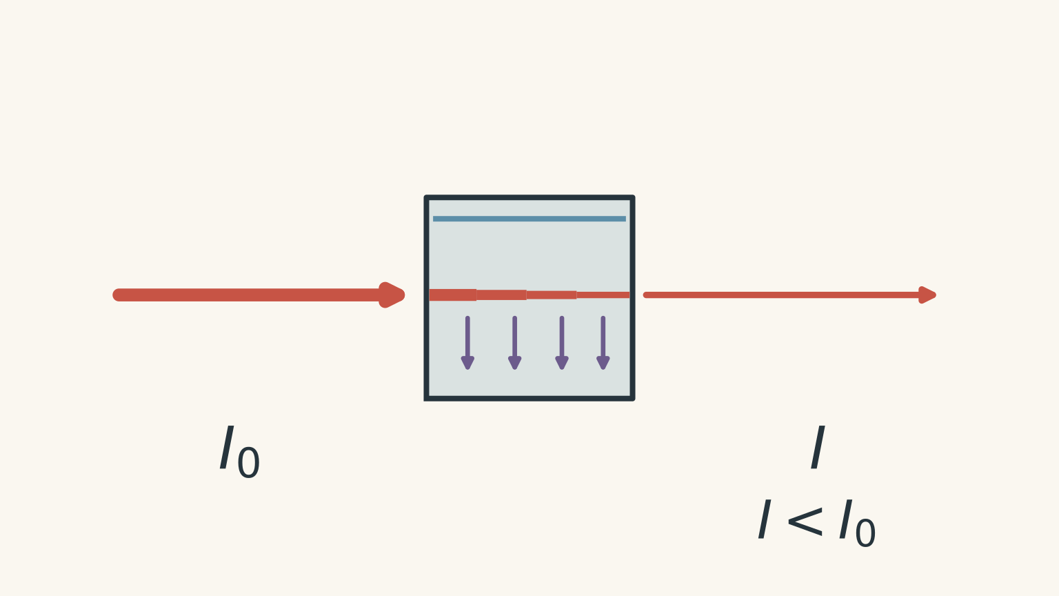
Call the intensity of the incident light \(I_0\) and the intensity transmitted through the sample \(I\).
If almost all the light passes through, the sample has absorbed very little. If only a small fraction gets through, the sample has absorbed strongly.
Before going further, predict this: if you double the concentration of an absorbing species while keeping everything else the same, what should happen?
There are now roughly twice as many absorbing particles in the beam’s path, so you expect more light to be absorbed. That intuition is correct, but the relationship is easiest to use through a quantity called absorbance.
02Transmittance and absorbance
The transmittance, \(T\), is the fraction of incident light that passes through the sample:
\[ T=\frac{I}{I_0} \]
For example, if 40% of the incoming light is transmitted,
\[ T=0.40 \]
Absorbance, \(A\), is defined by
\[ A=-\log_{10}(T) \]
or equivalently,
\[ A=\log_{10}\left(\frac{I_0}{I}\right) \]
Absorbance has no unit.
This logarithm may look like an unnecessary complication. It earns its place because absorbance, under suitable conditions, has a simple relationship with concentration.
Suppose 10% of the light is transmitted:
\[ A=-\log_{10}(0.10)=1.00 \]
If only 1% is transmitted:
\[ A=-\log_{10}(0.01)=2.00 \]
So an absorbance of 2 does not mean twice as much light was absorbed as at an absorbance of 1. The underlying intensity relationship is logarithmic.
That is a common trap. Absorbance is the convenient scale used for concentration measurements; it is not itself “percentage absorbed”.
03Why different substances absorb different wavelengths
White light contains a range of wavelengths. A coloured species does not absorb all of them equally.
Its electrons can absorb photons whose energies match allowed electronic energy changes. Because photon energy depends on wavelength,
\[ E=\frac{hc}{\lambda} \]
where:
- \(E\) is photon energy in joules,
- \(h\) is Planck’s constant,
- \(c\) is the speed of light in metres per second,
- \(\lambda\) is wavelength in metres.
Different species therefore tend to produce different patterns of absorbance across the ultraviolet and visible regions.
A UV-visible spectrophotometer can scan across wavelengths and produce an absorption spectrum: absorbance plotted against wavelength.
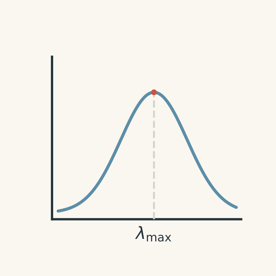
The wavelength at which absorbance is greatest is called \(\lambda_{\text{max}}\).
Why measure near \(\lambda_{\text{max}}\)?
Suppose a species absorbs weakly at 500 nm but strongly at 620 nm. A small change in concentration will cause a larger change in measured absorbance at 620 nm.
That makes the measurement more sensitive.
There is another practical advantage. Near the top of a broad absorption peak, a tiny wavelength error usually changes the absorbance less than it would on a steep side of the peak.
So, for quantitative analysis, a suitable wavelength is often chosen near \(\lambda_{\text{max}}\).
04Colour seen and colour absorbed are not the same thing
A blue solution looks blue because blue wavelengths are reaching your eyes. It has generally absorbed more strongly in another part of the visible spectrum.
So don’t reason:
“The solution is blue, therefore it absorbs blue light most strongly.”
That reverses the process.
The colour you observe mainly comes from the wavelengths that are transmitted through the solution, while the absorption spectrum records the wavelengths removed from the beam.
A rough complementary-colour model can help, but real spectra are broad, and colour perception depends on the whole transmitted spectrum. Treat the complementary-colour idea as a useful first model, not an exact identification method.
05Using a spectrum to identify a species
Suppose an unknown sample gives a strong absorption peak near the same wavelength as a known metal complex.
That is evidence that the complex may be present.
But one matching peak is not automatically proof. Different substances can have overlapping absorption bands, and mixtures can produce combined spectra.
Identification becomes stronger when the overall absorption pattern matches a reference under the same relevant conditions.
This gives UV-visible spectrophotometry two related jobs:
| Question | Useful measurement |
|---|---|
| What absorbing species might be present? | Position and shape of absorption bands |
| How much of a known species is present? | Absorbance at a selected wavelength |
The second job requires calibration.
06Why concentration changes absorbance
Picture a cuvette as a hallway full of students who keep trying to high-five every photon walking through.
Increasing the concentration is like putting more students in the hallway. Increasing the path length is like making the hallway longer. Either way, a photon has more opportunities to be intercepted.
The analogy is useful because it captures why concentration and path length both matter. It breaks down because real absorption is governed by quantum transitions, not photons being physically grabbed by tiny people.
Under appropriate conditions, the relationship is described by the Beer-Lambert law:
\[ A=\varepsilon bc \]
where:
- \(A\) is absorbance,
- \(\varepsilon\) is the molar absorption coefficient, usually in \(\text{L mol}^{-1}\text{ cm}^{-1}\),
- \(b\) is the path length through the sample in cm,
- \(c\) is concentration in \(\text{mol L}^{-1}\).
At a fixed wavelength, for the same species and the same cuvette path length, \(\varepsilon\) and \(b\) are constant. Therefore,
\[ A\propto c \]
This is the reason a calibration graph can work.
07Calibration turns absorbance into concentration
A spectrophotometer directly gives you absorbance. It does not magically know the concentration of an unknown solution.
You teach it the relationship first.
Prepare several standard solutions whose concentrations are known. Measure their absorbances under the same conditions. Plot absorbance against concentration.
For example:
| Concentration, \(c\) (\(\text{mol L}^{-1}\)) | Absorbance, \(A\) |
|---|---|
| \(1.00\times10^{-5}\) | 0.125 |
| \(2.00\times10^{-5}\) | 0.247 |
| \(3.00\times10^{-5}\) | 0.376 |
| \(4.00\times10^{-5}\) | 0.497 |
| \(5.00\times10^{-5}\) | 0.623 |
The values are close to a straight line.
A line of best fit might be represented by
\[ A=1.25\times10^4 c \]
where \(c\) is in \(\text{mol L}^{-1}\).
Now an unknown absorbance can be converted into a concentration.
If you’d like more practice specifically with calibration curves and concentration calculations, tutorgum’s colourimetry guide develops the same core relationship in more detail.
Worked example: Find concentration from absorbance
A coloured complex has a calibration relationship
\[ A=8.40\times10^3c \]
where \(c\) is in \(\text{mol L}^{-1}\). An unknown solution gives an absorbance of 0.462 at the wavelength used for calibration. Determine its concentration.
Step 1
The measured absorbance \(A\) is related to concentration \(c\). We know \(A=0.462\).
Step 2
\[ 0.462=(8.40\times10^3)c \]
Step 3
\[ c=\frac{0.462}{8.40\times10^3} =5.50\times10^{-5}\text{ mol L}^{-1} \]
The concentration is therefore
\[ \boxed{5.50\times10^{-5}\text{ mol L}^{-1}} \]
The result means that the unknown has the concentration expected to produce an absorbance of 0.462 under the same experimental conditions used for the standards.
That last phrase matters.
08The unknown and standards must be comparable
A calibration only makes sense if the standards and unknown are being compared fairly.
Keep these conditions consistent:
- the wavelength used,
- the chemical form of the absorbing species,
- the solvent and relevant solution conditions, such as pH,
- the cuvette path length,
- the instrument setup,
- and the preparation procedure where possible.
Imagine calibrating the colour of cordial using one glass that is 1 cm wide, then measuring your unknown through a glass 4 cm wide. The second sample gives the light a much longer journey through the solution. A larger absorbance would not necessarily mean a greater concentration.
This is why standard cuvettes have a fixed optical path length, commonly 1 cm.
09What the blank actually does
Even a solution containing none of the analyte may absorb or scatter a little light.
The solvent absorbs some radiation. Reagents may absorb. The cuvette itself affects the beam.
A blank contains the components that should not be attributed to the analyte. It is used to establish the instrumental baseline.
Suppose your analyte is dissolved in water with another reagent added to every standard and sample. A suitable blank normally contains the water and reagent but not the analyte being measured.
Think of it as measuring the background noise before trying to hear one person’s voice.
The analogy breaks if you imagine the spectrophotometer literally subtracting a fixed amount of “colour” from every sample. The instrument is establishing a reference for transmitted intensity, and the exact procedure depends on the instrument.
10Calibration curves are measured relationships, not decorative straight lines
In ideal Beer-Lambert behaviour, a graph of absorbance against concentration is linear.
Real data will usually scatter slightly because measurements have uncertainty. You therefore use a line of best fit rather than joining each point dot-to-dot.
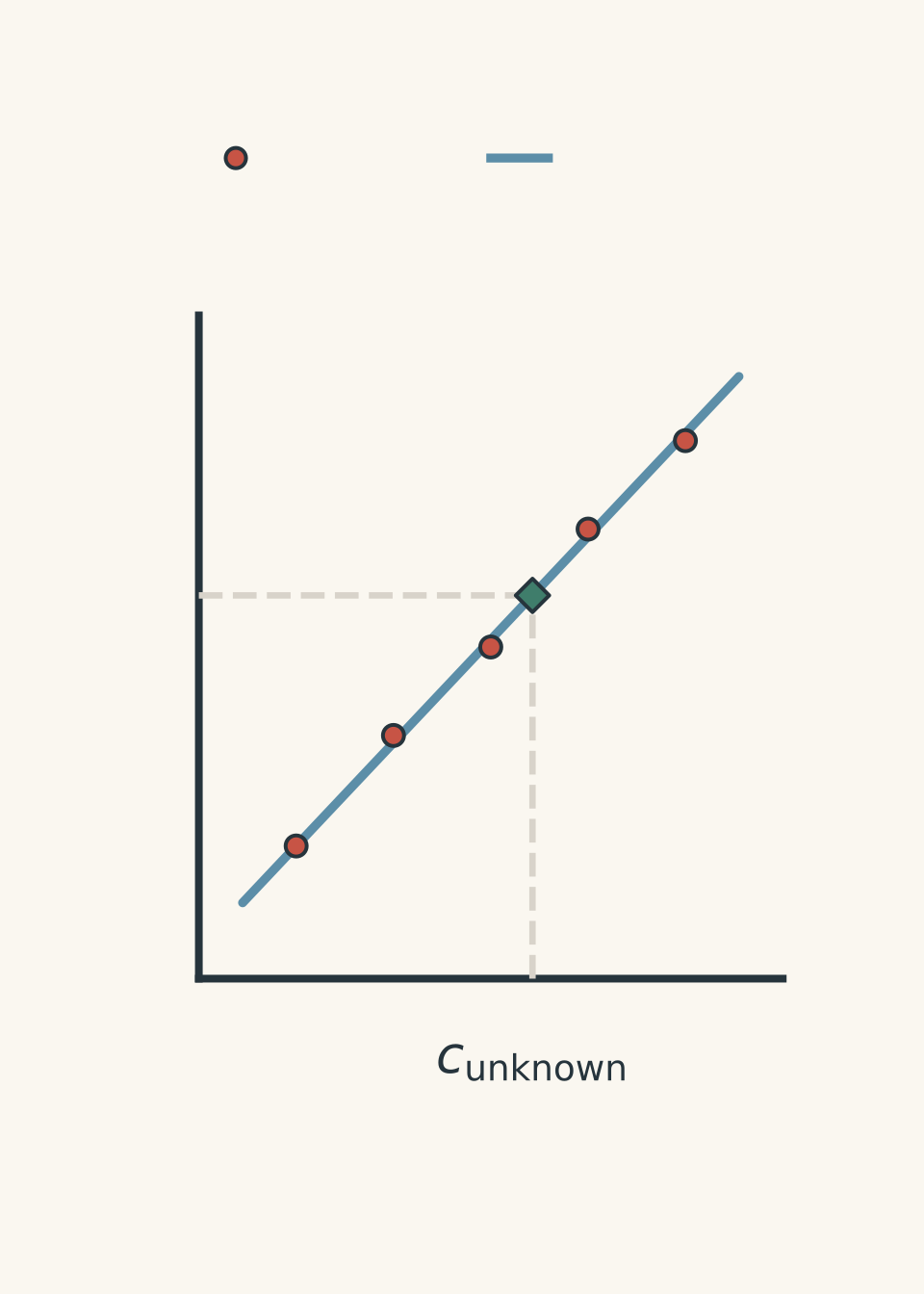
A calibration equation may include an intercept:
\[ A=mc+b \]
Here:
- \(A\) is absorbance,
- \(c\) is concentration,
- \(m\) is the gradient or sensitivity,
- \(b\) is the \(A\)-axis intercept.
In a simple ideal model with perfect blank correction, \(b\) would be zero. Real experimental data can give a small non-zero intercept.
Don’t automatically force the line through the origin unless there is a justified reason to do so.
11Interpolation is safer than extrapolation
Suppose your standards cover absorbances from 0.10 to 0.75, but the unknown gives \(A=1.18\).
It is tempting to extend the line and calculate a concentration anyway.
The problem is that you have not demonstrated that your calibration remains valid at that higher concentration. Beer-Lambert behaviour can deviate from linearity, and instrument performance may become less reliable when very little light reaches the detector.
A better approach is usually to dilute the unknown until its absorbance lies inside the calibration range, determine the diluted concentration, then undo the dilution mathematically.
Worked example: Measure an unknown after dilution
A calibration for an ion at 525 nm is
\[ A=(2.60\times10^3)c+0.006 \]
where \(c\) is measured in \(\text{mol L}^{-1}\).
An unknown solution initially gives an absorbance above the calibrated range. A 10.00 mL portion is diluted to 50.00 mL. The diluted solution has an absorbance of 0.552.
Determine the concentration of the original solution.
Step 1
\[ 0.552=(2.60\times10^3)c+0.006 \]
\[ 0.546=(2.60\times10^3)c \]
\[ c=\frac{0.546}{2.60\times10^3} =2.10\times10^{-4}\text{ mol L}^{-1} \]
This is the concentration after dilution.
Step 2
A 10.00 mL portion was diluted to 50.00 mL:
\[ \text{dilution factor}=\frac{50.00}{10.00}=5.000 \]
Step 3
\[ c_{\text{original}} =(2.10\times10^{-4})(5.000) =1.05\times10^{-3}\text{ mol L}^{-1} \]
So the original concentration was
\[ \boxed{1.05\times10^{-3}\text{ mol L}^{-1}} \]
Dilution did not remove analyte from the transferred 10.00 mL sample. It increased the volume and therefore lowered the concentration. Once the diluted concentration is measured, the dilution factor reconstructs the original value.
12The most tempting misconception: darker always means more concentrated
For two solutions containing the same absorbing species, measured under identical conditions at an appropriate wavelength, greater absorbance usually indicates greater concentration within the valid linear range.
But “darker means more concentrated” is not a general law.
A darker-looking solution could involve:
- a different chemical species,
- a different path length,
- a different wavelength distribution,
- multiple absorbing species,
- changed pH causing the species to change form,
- or a concentration outside the reliable calibration range.
UV-visible analysis works because experimental conditions are controlled. Colour alone is not enough.
This becomes especially important in environmental analysis, where other species in a sample can interfere. The broader problem of turning analytical measurements into defensible conclusions is developed in tutorgum’s environmental chemical monitoring guide.
13What can make Beer-Lambert behaviour fail?
The neat statement \(A=\varepsilon bc\) has conditions attached.
Very concentrated solutions
At higher concentrations, interactions between particles can change their absorbing behaviour. The simple proportional relationship may no longer hold closely.
Chemical changes in the sample
Suppose the substance exists in two forms depending on pH, and the two forms have different absorption spectra.
Changing the pH then changes more than concentration. It changes which species are present.
A calibration prepared at one pH may no longer correctly describe an unknown at another.
Stray light and instrumental limits
If absorbance is extremely high, very little intended light reaches the detector. Small amounts of stray light can then become significant relative to the transmitted beam.
Scattering
Suspended particles can scatter light away from the detector. The instrument may interpret some of that lost light as absorption, producing an absorbance that is too high.
This is one reason a cloudy sample deserves suspicion.
14A practical decision process
When you are given UV-visible data in an HSC-style problem, work through the reasoning in this order:
- Identify the wavelength and species being measured. Ask whether the measurement is selective enough for the intended analyte.
- Check the calibration range. An unknown should ideally fall within the range established by standards.
- Use the calibration equation or graph. If \(A=mc+b\), rearrange to \(c=(A-b)/m\).
- Account for any dilution. The spectrophotometer measures the solution actually placed in the cuvette, not its earlier concentration.
- Check units. Convert between \(\text{mol L}^{-1}\), \(\text{g L}^{-1}\), or \(\text{mg L}^{-1}\) only when required.
- Judge whether the calibration is chemically valid. Different pH, species, matrix, or excessive absorbance can undermine a numerically tidy answer.
A calculator can handle step 3. Most of the chemistry is hiding in steps 1, 2, and 6.
15Questions and solutions
Question 1
A solution containing a coloured metal complex is measured at its \(\lambda_{\text{max}}\). Its calibration equation is
\[ A=(4.80\times10^3)c+0.004 \]
where \(c\) is in \(\text{mol L}^{-1}\).
An unknown gives an absorbance of 0.388. Calculate its concentration.
Solution 1
The concentration is \(\boxed{8.00\times10^{-5}\text{ mol L}^{-1}}\).
The calibration equation directly relates absorbance to concentration:
\[ A=(4.80\times10^3)c+0.004 \]
Substitute \(A=0.388\):
\[ \begin{aligned} 0.388&=(4.80\times10^3)c+0.004\\ 0.384&=(4.80\times10^3)c\\ c&=\frac{0.384}{4.80\times10^3}\\ &=8.00\times10^{-5}\text{ mol L}^{-1} \end{aligned} \]
The small intercept must be included. A tempting shortcut is to use \(A=mc\) and ignore the 0.004, but the supplied calibration tells us that the measured relationship has a non-zero intercept.
Question 2
A water sample containing a coloured ion gives an absorbance of 1.36. The calibration standards used for the analysis had absorbances between 0.08 and 0.82.
A student substitutes \(A=1.36\) into the linear calibration equation and reports the resulting concentration.
Explain why this result is less defensible than one obtained by diluting the sample and remeasuring it. Describe how the final concentration should be determined after dilution.
Solution 2
The sample should be diluted until its measured absorbance lies within the established calibration range, then the calculated diluted concentration should be multiplied by the appropriate dilution factor.
The student’s calculation is an extrapolation. The standards only establish the relationship between concentration and absorbance over the measured range corresponding to absorbances from 0.08 to 0.82.
Using the line at \(A=1.36\) assumes that the same linear relationship continues well beyond the experimental evidence. That may fail because concentrated solutions can deviate from ideal Beer-Lambert behaviour and because highly absorbing samples transmit very little light, making instrumental effects more important.
After dilution:
- measure the diluted sample’s absorbance within the calibration range;
- use the calibration equation to determine \(c_{\text{diluted}}\);
- determine the dilution factor,
\[ \text{dilution factor}= \frac{V_{\text{final}}}{V_{\text{aliquot}}}; \]
- calculate
\[ c_{\text{original}} =c_{\text{diluted}} \times \frac{V_{\text{final}}}{V_{\text{aliquot}}}. \]
The tempting argument is that a straight calibration line can simply be extended forever. The problem is experimental rather than algebraic: linearity outside the calibrated region has not been demonstrated.
Question 3
A coloured species \(X\) is analysed using standards prepared at pH 10. Their calibration equation at 610 nm is
\[ A=(6.20\times10^3)c+0.003 \]
where \(c\) is in \(\text{mol L}^{-1}\).
An unknown sample at pH 5 gives \(A=0.499\). A student calculates
\[ c=\frac{0.499-0.003}{6.20\times10^3} =8.00\times10^{-5}\text{ mol L}^{-1}. \]
It is then discovered that \(X\) undergoes an acid-base reaction, and its acidic form has a different absorption spectrum from its basic form.
Evaluate the student’s concentration.
Solution 3
The numerical calculation is correct for the calibration equation, but \(\boxed{8.00\times10^{-5}\text{ mol L}^{-1}}\) cannot be accepted as a reliable concentration of total \(X\) without further information.
The student has correctly performed:
\[ \begin{aligned} c&=\frac{A-b}{m}\\ &=\frac{0.499-0.003}{6.20\times10^3}\\ &=8.00\times10^{-5}\text{ mol L}^{-1}. \end{aligned} \]
The problem is the chemistry behind the calibration.
The standards were prepared at pH 10, but the unknown is at pH 5. If \(X\) changes protonation state with pH and its acidic and basic forms have different absorption spectra, the molar absorption coefficient \(\varepsilon\) at 610 nm is not necessarily the same in the standards and unknown.
Therefore the calibration relationship
\[ A=\varepsilon bc \]
is being applied with a potentially different value of \(\varepsilon\).
The tempting conclusion is that matching an absorbance to a calibration line must give the concentration. That only works when the unknown behaves spectroscopically like the standards. The sample should instead be adjusted to the same controlled chemical conditions as the standards, or calibrated using standards that reproduce the sample conditions.
Question 4
Five standards give the following results at 540 nm.
| Concentration (\(\text{mol L}^{-1}\)) | Absorbance |
|---|---|
| 0 | 0.081 |
| \(1.00\times10^{-5}\) | 0.142 |
| \(2.00\times10^{-5}\) | 0.201 |
| \(3.00\times10^{-5}\) | 0.262 |
| \(4.00\times10^{-5}\) | 0.321 |
The relationship is highly linear.
A student says:
“Because the graph is straight, the experiment obeys Beer-Lambert law perfectly, so the blank must have been prepared correctly.”
The zero-concentration standard was made using the same solvent as the other solutions, but it accidentally omitted a colour-forming reagent that was present at constant concentration in every non-zero standard and in every unknown.
Assess the student’s conclusion. Predict how this error could affect concentrations calculated using a calibration forced through the origin.
Solution 4
The student’s conclusion is incorrect. The straight line shows that the response is highly linear, but the large absorbance at zero analyte concentration reveals a substantial background contribution, and the incorrectly prepared blank fails to reproduce that background.
At zero analyte concentration the measured absorbance is 0.081, not close to zero. The important clue is that every actual sample contains a colour-forming reagent that the blank lacks.
The standards approximately increase by \(0.060\) absorbance units for every \(1.00\times10^{-5}\text{ mol L}^{-1}\) increase in analyte concentration. A suitable measured relationship is therefore roughly
\[ A\approx(6.0\times10^3)c+0.081. \]
The non-zero intercept is not evidence that concentration somehow exists when \(c=0\). It indicates a measured background absorbance.
If a student incorrectly forces the calibration through the origin, some of that background absorbance will be attributed to the analyte. The calculated concentrations will therefore generally be too high, particularly at low analyte concentrations where 0.081 is a large fraction of the total absorbance.
For example, a sample with \(A=0.201\) corresponds, using the measured relationship, to
\[ \begin{aligned} 0.201&=(6.0\times10^3)c+0.081\\ c&=\frac{0.120}{6.0\times10^3}\\ &=2.0\times10^{-5}\text{ mol L}^{-1}. \end{aligned} \]
If the entire absorbance of 0.201 were treated as analyte response, the concentration would be overestimated.
The tempting route is to equate “straight graph” with “perfect experiment”. Linearity only tells us that one variable changes predictably with another. A systematic error can itself be extremely consistent and produce a beautifully straight but misleading calibration.
Question 5
Two coloured species, \(X\) and \(Y\), can both be present in the same solution. Their absorption bands overlap.
Calibration experiments show that, under fixed conditions and using the same 1.00 cm cuvette, their absorbance contributions are:
| Species concentration | Absorbance at 450 nm | Absorbance at 600 nm |
|---|---|---|
| \(1.00\times10^{-4}\text{ mol L}^{-1}\) of \(X\) | 0.600 | 0.200 |
| \(1.00\times10^{-4}\text{ mol L}^{-1}\) of \(Y\) | 0.100 | 0.500 |
Assume that Beer-Lambert behaviour is linear and that, when \(X\) and \(Y\) are mixed, their absorbance contributions add.
An unknown mixture gives:
\[ A_{450}=0.440 \]
and
\[ A_{600}=0.380. \]
A student notices that \(X\) absorbs much more strongly at 450 nm than \(Y\) and concludes that the 450 nm measurement can be treated as if only \(X\) were present.
Determine the concentrations of both \(X\) and \(Y\), and explain why the student’s apparently reasonable shortcut fails.
Solution 5
The mixture contains
\[ \boxed{[X]=6.50\times10^{-5}\text{ mol L}^{-1}} \]
and
\[ \boxed{[Y]=5.00\times10^{-5}\text{ mol L}^{-1}}. \]
The key is that “absorbs more strongly” does not mean “absorbs exclusively”. Species \(Y\) still contributes to the absorbance at 450 nm, while \(X\) contributes at 600 nm.
Let
\[ x=\frac{[X]}{1.00\times10^{-4}\text{ mol L}^{-1}} \]
and
\[ y=\frac{[Y]}{1.00\times10^{-4}\text{ mol L}^{-1}}. \]
Because absorbances are assumed to add, the 450 nm measurement gives
\[ 0.600x+0.100y=0.440. \]
The 600 nm measurement gives
\[ 0.200x+0.500y=0.380. \]
Multiply the second equation by 3:
\[ 0.600x+1.500y=1.140. \]
Subtract the first equation:
\[ 1.400y=0.700 \]
so
\[ y=0.500. \]
Therefore,
\[ [Y]=(0.500)(1.00\times10^{-4}) =5.00\times10^{-5}\text{ mol L}^{-1}. \]
Substitute \(y=0.500\) into the first equation:
\[ \begin{aligned} 0.600x+0.100(0.500)&=0.440\\ 0.600x+0.050&=0.440\\ 0.600x&=0.390\\ x&=0.650. \end{aligned} \]
Thus,
\[ [X]=(0.650)(1.00\times10^{-4}) =6.50\times10^{-5}\text{ mol L}^{-1}. \]
Now consider the tempting shortcut. If the student pretended that all of the 450 nm absorbance came from \(X\), they would calculate
\[ x=\frac{0.440}{0.600}=0.733, \]
giving
\[ [X]=7.33\times10^{-5}\text{ mol L}^{-1}. \]
That is too high because part of the measured absorbance – 0.050 absorbance units in the actual mixture – came from \(Y\).
The deeper point is that an instrument measures the total effect on the light beam. It does not label individual absorbed photons as “caused by \(X\)” or “caused by \(Y\)”. Selectivity comes from the pattern across wavelengths. When spectra overlap, measurements at multiple wavelengths can sometimes separate contributions that one wavelength cannot.
16What UV-visible spectrophotometry lets you do next
The central chain is now:
\[ \text{species} \rightarrow \text{wavelength-dependent absorption} \rightarrow \text{absorbance} \rightarrow \text{calibration} \rightarrow \text{concentration}. \]
For identification, look at where absorption occurs and recognise that a spectral match is evidence rather than automatic proof.
For quantification, control the chemical conditions, measure at a suitable wavelength, calibrate using known standards, keep the unknown within the validated range, and account for dilution.
That same reasoning carries into real analytical chemistry. The next useful question is no longer simply “What concentration did I calculate?” It is “Does this measurement genuinely represent the species I think I measured?” That is where interference, sample preparation, uncertainty, and the quality of analytical evidence become just as important as the calibration equation.