
Digital Probes for Acid-Base Analysis in HSC Chemistry
Learn how pH and conductivity probes collect, process, and evaluate acid-base data. Includes titration examples, data interpretation, errors, and challenging HSC-style questions.
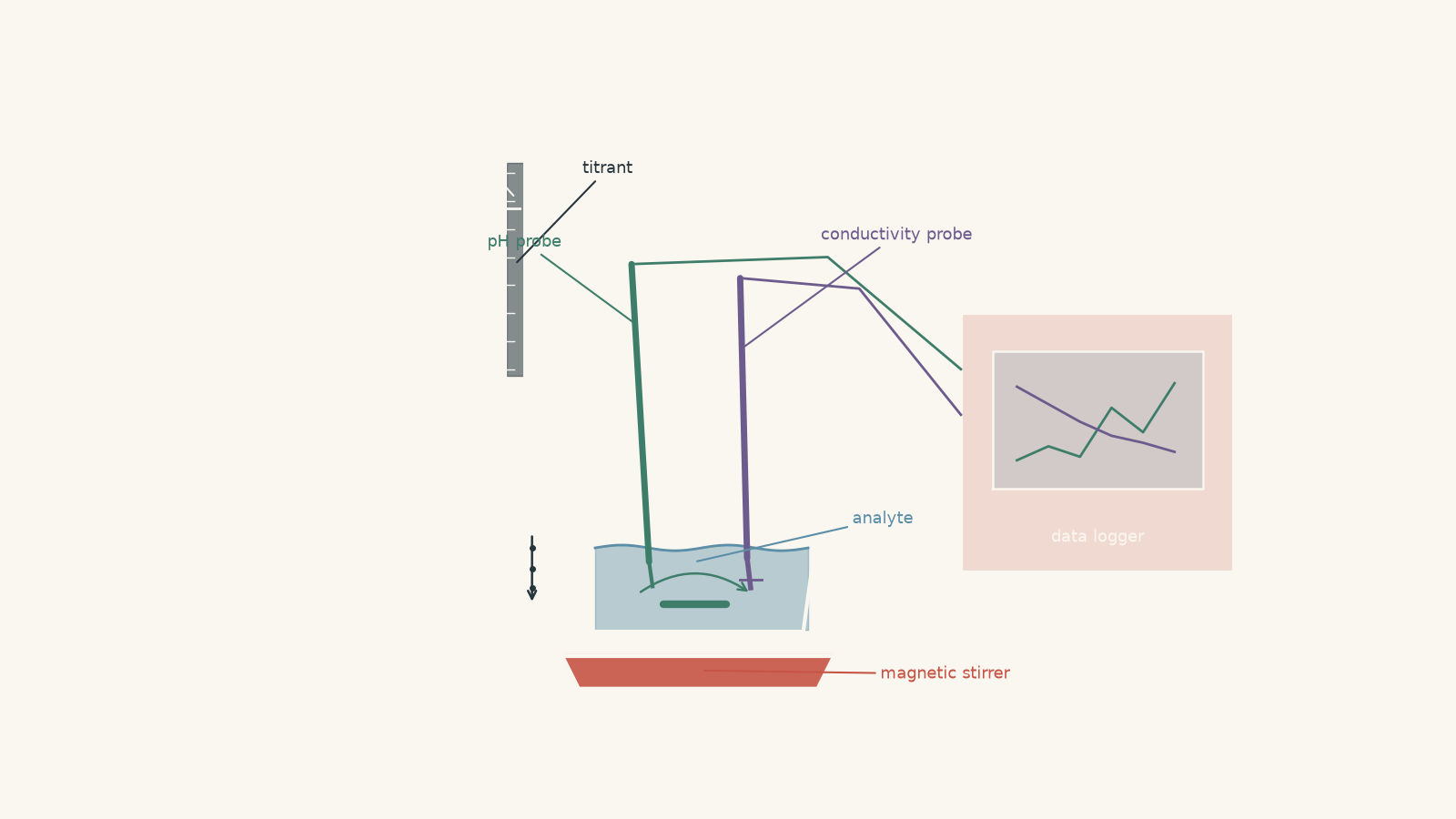
A colour change can tell you roughly where a titration ends. It cannot tell you what happened on the way there. A digital probe can record hundreds of measurements as an acid is neutralised, revealing changes that your eyes would completely miss.
Suppose you titrate hydrochloric acid with sodium hydroxide while recording both pH and conductivity. Before seeing the graphs, predict this: will the two probes trace the same shape because they are both responding to ions?
They will not. A pH probe responds specifically to acidity, while a conductivity probe responds to all mobile ions in the solution. That difference is exactly why using the two together can be so useful.
01What is a digital probe actually measuring?
The important habit is to separate three stages:
- collect: obtain measurements from the solution,
- process: turn those measurements into useful graphs, calculations, or endpoint estimates,
- evaluate: decide how trustworthy the result is.
A computer doing the processing does not remove the need for chemistry. It just makes bad chemistry happen faster if you feed it bad data.
A pH probe does not literally detect a number called pH
A typical laboratory pH probe contains a glass electrode whose electrical potential changes with hydrogen ion activity. The meter measures a voltage and converts it to pH using calibration data.
For HSC calculations, we normally use the approximation
\[
\text{pH}=-\log_{10}[\ce{H3O+}]
\]
where \([\ce{H3O+}]\) is the hydronium ion concentration in \(\text{mol L}^{-1}\).
Strictly, pH depends on hydronium ion activity, not simply concentration. That distinction becomes important in concentrated or high-ionic-strength solutions. For ordinary HSC calculations, treating activity as concentration is the useful model.
The logarithm matters. A change from pH 4 to pH 3 is not a tiny change of one unit. It represents a tenfold increase in hydronium ion concentration.
A conductivity probe asks a different question
Conductivity measures how easily electrical charge can move through the solution.
In an aqueous solution, that charge is carried by ions. More mobile ions generally mean greater conductivity.
A conductivity probe therefore responds to ions such as:
\[
\ce{H3O+},\ \ce{OH-},\ \mathrm{Na}^{+},\ \mathrm{Cl}^{-},\ \ce{CH3COO-}
\]
and any other ions present.
Most laboratory conductivity meters measure the electrical conductance between electrodes, then use the geometry of the probe, represented by a cell constant, to calculate conductivity. Conductivity may be reported in units such as \(\text{S m}^{-1}\), \(\text{mS cm}^{-1}\), or \(\mu\text{S cm}^{-1}\).
Why pH and conductivity are not interchangeable
Imagine three solutions:
| Solution | pH behaviour | Conductivity behaviour |
|---|---|---|
| Dilute \(\ce{HCl}\) | Acidic | Conducts because \(\ce{H3O+}\) and \(\mathrm{Cl}^{-}\) are present |
| \(\ce{NaCl}\) solution | Approximately neutral | Can conduct strongly because \(\mathrm{Na}^{+}\) and \(\mathrm{Cl}^{-}\) are present |
| Pure water | Approximately neutral | Very low conductivity because very few ions are present |
So a high conductivity does not mean a solution is strongly acidic.
That is a very tempting misconception because acids contain ions, and stronger acids often do conduct well. The missing idea is that conductivity is not selective. A conductivity probe does not care whether an ion is making the solution acidic.
02Collecting useful probe data
Digital instruments give precise-looking numbers. A display showing pH 4.327 is not evidence that the true pH is known to three decimal places.
The quality of the data still depends on how the experiment is performed.
Calibrate before trusting the reading
A pH meter should be calibrated using buffer solutions with known pH values. Ideally, the calibration points should cover the pH range being measured.
For example, if you expect measurements mostly between pH 4 and pH 10, suitable calibration buffers might include pH 4, 7, and 10.
The basic sequence is:
- calibrate the probe using appropriate standard buffers,
- rinse the probe with deionised water between solutions,
- gently blot away excess water rather than scrubbing the sensing surface,
- immerse the sensing region correctly,
- allow the reading to stabilise,
- record the temperature where it matters.
A conductivity probe is similarly calibrated using a standard solution of known conductivity.
Calibration corrects the relationship between the instrument’s electrical signal and the value displayed to you. It cannot fix contamination, incorrect titrant concentration, a badly read burette, or a sample prepared incorrectly.
Keep the solution mixed
Suppose a drop of concentrated \(\ce{NaOH}\) falls beside the pH electrode during a titration. For a moment, the probe may be sitting in a tiny region with far more \(\ce{OH-}\) than the rest of the beaker.
The displayed pH could jump even though the whole solution has not yet reached that pH.
Gentle, continuous stirring helps make the measured solution representative of the whole sample.
The stirring should not be so violent that solution splashes from the vessel or a vortex exposes part of the probe.
Give the probe time to respond
A chemical change can occur faster than the instrument reaches a stable reading.
This matters particularly near a titration endpoint, where a very small volume of titrant can cause a large pH change.
If you add 1.00 mL portions, immediately record the displayed number, and keep going, a data logger cannot recreate the measurements you failed to collect.
Near an endpoint, smaller volume additions and adequate stabilisation time are usually more useful.
Record the independent variable properly
For a titration, pH should normally be plotted against volume of titrant added, not simply against time.
Why?
Imagine that you pause for 30 seconds at one point and then add titrant rapidly for the next 30 seconds. Equal time intervals no longer correspond to equal titrant volumes.
Time is only a useful substitute if titrant is being delivered at a known, controlled rate.
03Processing pH data
The simplest useful output is a graph of pH against titrant volume.
For a strong acid titrated with a strong base, the curve typically has:
- a low initial pH,
- a gradual increase,
- a very steep change near equivalence,
- a high-pH region after excess base is present.
The equivalence point is the stoichiometric point where the reacting acid and base have been added in the required mole ratio.
For
\[
\ce{HCl + NaOH -> NaCl + H2O}
\]
the mole ratio is \(1:1\), so at equivalence
\[
n(\ce{HCl})=n(\ce{NaOH})
\]
Do not quietly replace the words “equivalence point” with “pH 7”.
A strong acid-strong base titration is approximately pH 7 at equivalence at \(25^\circ\text{C}\). A weak acid titrated with a strong base has an equivalence point above pH 7 because the conjugate base produced can react with water.
The equivalence point is defined by stoichiometry, not by a particular pH number.
Worked example: finding concentration from a digital pH curve
A student titrates \(25.00\text{ mL}\) of hydrochloric acid with \(0.1000\text{ mol L}^{-1}\) sodium hydroxide. A pH probe produces the following data near the steep section of the curve.
| \(\ce{NaOH}\) added (mL) | pH |
|---|---|
| 24.2 | 2.79 |
| 24.6 | 3.09 |
| 24.8 | 3.40 |
| 25.0 | 7.00 |
| 25.2 | 10.60 |
| 25.4 | 10.90 |
Estimate the concentration of the original hydrochloric acid.
Step 1
The enormous pH change occurs around \(25.0\text{ mL}\). The curve is centred on approximately
\[
V_{\text{eq}}=25.0\text{ mL}=0.0250\text{ L}
\]
Step 2
\[
\ce{HCl + NaOH -> NaCl + H2O}
\]
The mole ratio is \(1:1\), so
\[
n(\ce{HCl})=n(\ce{NaOH})
\]
Step 3
\[
\begin{aligned}
n(\ce{NaOH})
&=cV\\
&=(0.1000\text{ mol L}^{-1})(0.0250\text{ L})\\
&=2.50\times10^{-3}\text{ mol}
\end{aligned}
\]
Therefore the original sample contained \(2.50\times10^{-3}\text{ mol}\) of \(\ce{HCl}\).
Step 4
\[
\begin{aligned}
c(\ce{HCl})
&=\frac{n}{V}\\
&=\frac{2.50\times10^{-3}\text{ mol}}{0.02500\text{ L}}\\
&=0.100\text{ mol L}^{-1}
\end{aligned}
\]
The pH curve therefore indicates an HCl concentration of approximately \(0.100\text{ mol L}^{-1}\).
The probe did not directly measure that concentration. It helped us identify an equivalence volume, and the concentration then came from stoichiometry.
Processing the steep section more carefully
With closely spaced data, software can calculate an approximate gradient:
\[
\frac{\Delta\text{pH}}{\Delta V}
\]
where \(\Delta\text{pH}\) is the change in pH and \(\Delta V\) is the corresponding change in titrant volume.
The largest gradient occurs near the inflection region of the titration curve and can provide a more objective estimate of the endpoint than simply staring at the graph and saying, “That bit looks pretty vertical.”
There is still a limitation. If your measurements are 2 mL apart, numerical processing cannot magically locate an endpoint to \(0.01\text{ mL}\). The raw data must contain enough resolution in the first place.
04Processing conductivity data
Now predict what happens during a strong acid-strong base titration.
At the beginning, an \(\ce{HCl}\) solution contains \(\ce{H3O+}\) and \(\mathrm{Cl}^{-}\). As \(\ce{NaOH}\) is added, the reaction
\[
\ce{H3O+ + OH- -> 2H2O}
\]
removes hydronium ions.
The \(\mathrm{Na}^{+}\) ions remain in solution, so before equivalence the highly mobile \(\ce{H3O+}\) ions are progressively being replaced by less mobile \(\mathrm{Na}^{+}\) ions. Conductivity therefore usually decreases.
At equivalence, essentially all the original excess \(\ce{H3O+}\) has been neutralised.
Beyond equivalence, additional \(\ce{NaOH}\) leaves both \(\mathrm{Na}^{+}\) and \(\ce{OH-}\) in solution. Conductivity begins to rise.
A graph can therefore produce two regions with different slopes whose intersection gives an estimate of the equivalence volume.
What changes for a weak acid?
Consider ethanoic acid:
\[
\ce{CH3COOH <=> H+ + CH3COO-}
\]
Only a fraction is ionised before the titration. Its initial conductivity is therefore much lower than that of an equally concentrated strong acid such as HCl.
When \(\ce{NaOH}\) is added,
\[
\ce{CH3COOH + OH- -> CH3COO- + H2O}
\]
and the solution accumulates \(\mathrm{Na}^{+}\) and \(\ce{CH3COO-}\).
So the conductivity may increase before equivalence rather than fall. After equivalence, excess \(\ce{OH-}\) produces a steeper increase.
This is a good example of why memorising “conductivity falls until the endpoint” is dangerous. That trend belongs to a particular chemical system, not to titration as a whole.
Worked example: finding an endpoint from conductivity lines
A \(20.00\text{ mL}\) sample of a monoprotic strong acid is titrated with \(0.0800\text{ mol L}^{-1}\) \(\ce{NaOH}\).
After collecting conductivity measurements, a student fits straight lines to the regions before and after the conductivity minimum. The equations are
\[
\kappa=8.20-0.260V
\]
before equivalence, and
\[
\kappa=-5.70+0.295V
\]
after equivalence.
Here, \(\kappa\) is conductivity in \(\text{mS cm}^{-1}\), and \(V\) is the volume of \(\ce{NaOH}\) added in mL.
Find the acid concentration.
Step 1
At the intersection, both expressions for conductivity are equal:
\[
8.20-0.260V=-5.70+0.295V
\]
Rearranging,
\[
\begin{aligned}
13.90&=0.555V\\
V&=25.0\text{ mL}
\end{aligned}
\]
So the estimated equivalence volume is
\[
V_{\text{eq}}=25.0\text{ mL}=0.0250\text{ L}
\]
Step 2
\[
\begin{aligned}
n(\ce{NaOH})
&=cV\\
&=(0.0800\text{ mol L}^{-1})(0.0250\text{ L})\\
&=2.00\times10^{-3}\text{ mol}
\end{aligned}
\]
Step 3
For a monoprotic strong acid represented as \(\ce{HA}\),
\[
\ce{HA + NaOH -> NaA + H2O}
\]
so
\[
n(\ce{HA})=2.00\times10^{-3}\text{ mol}
\]
Step 4
\[
\begin{aligned}
c(\ce{HA})
&=\frac{2.00\times10^{-3}\text{ mol}}{0.02000\text{ L}}\\
&=0.100\text{ mol L}^{-1}
\end{aligned}
\]
The conductivity data therefore give an acid concentration of approximately \(0.100\text{ mol L}^{-1}\).
Using fitted regions is often better than choosing one noisy reading and declaring it the minimum. Several measurements contribute to the endpoint estimate.
05Choosing between pH and conductivity
Neither probe is automatically “better”. The better measurement is the one that responds clearly to the chemical change you need to analyse.
| Question | pH probe | Conductivity probe |
|---|---|---|
| How acidic is the solution? | Directly useful | Not specific enough |
| Where is the steep pH change in a titration? | Very useful | May also help |
| Is the total ionic environment changing? | Limited | Very useful |
| Is a neutral salt present? | May barely respond | Often responds strongly |
| Can a coloured solution be analysed without an indicator colour change? | Yes | Often yes |
| Does the display alone identify the reacting species? | No | No |
Digital methods are particularly useful when a visual indicator is difficult to observe, when the full titration curve matters, or when you want a large data set rather than one final colour judgement.
For the wider use of these measurements in analytical chemistry, including choosing titration methods for real samples, see tutorgum’s guide to industrial acid-base analysis and titration.
06Evaluating the data rather than worshipping the decimal places
A digital instrument can improve resolution and reduce some forms of human judgement. It also introduces its own possible errors.
Accuracy, precision, and resolution are different
Accuracy is how close a result is to the accepted or true value.
Precision is how closely repeated measurements agree with one another.
Resolution is the smallest change the instrument can display or detect.
A probe that repeatedly reads pH 7.42 for a pH 7.00 buffer may be highly precise but inaccurate.
Displaying pH to 0.001 also does not prove an accuracy of \(\pm0.001\).
Calibration error can shift every result
Suppose a pH probe reads every solution about 0.30 pH units too high because it was badly calibrated.
Repeated measurements could form a beautifully smooth curve. The data would still contain a systematic error.
This matters when interpreting absolute pH values.
Interestingly, a constant vertical offset does not necessarily destroy every conclusion from the experiment. The position of the steepest section of a titration curve may remain close to the same titrant volume even if the whole pH curve is shifted upwards.
That becomes important in the final practice question.
Temperature matters
Both pH measurements and conductivity can depend on temperature.
Conductivity is particularly sensitive because the movement of ions changes with temperature. Many meters apply automatic temperature compensation, but that feature is itself based on a model.
If different samples are measured at substantially different temperatures, you should not silently treat their conductivity values as perfectly comparable.
Contamination affects the two probes differently
Imagine accidentally adding sodium chloride to an acid sample.
In the simple HSC model, \(\ce{NaCl}\) does not significantly change the acid’s amount of \(\ce{H3O+}\), so the pH may change little.
Conductivity, however, can increase substantially because extra \(\mathrm{Na}^{+}\) and \(\mathrm{Cl}^{-}\) ions are now carrying charge.
That difference can actually help you diagnose the experiment.
It is a little like asking two witnesses different questions. The pH probe is obsessed with one part of the story: acidity. The conductivity probe is the nosy friend who reports everyone charged who showed up. The analogy breaks because ions are not choosing to gossip, and conductivity also depends on their mobility, concentration, and temperature.
Dilution can alter conductivity even without new chemistry
Every time titrant is added, the total solution volume increases.
That means ions already present become more dilute.
For many titrations the chemical changes dominate the shape of the conductivity graph, but a large concentration of spectator ions can make dilution important.
A simple approximate dilution correction sometimes used when processing conductivity titration data is
\[
\kappa_{\text{corr}}
=
\kappa_{\text{meas}}
\left(\frac{V_0+V}{V_0}\right)
\]
where:
- \(\kappa_{\text{meas}}\) is the measured conductivity,
- \(\kappa_{\text{corr}}\) is the conductivity corrected approximately for dilution,
- \(V_0\) is the initial sample volume,
- \(V\) is the titrant volume added.
This assumes the ionic conductivities behave approximately consistently over the concentration range. It is a processing model, not an exact law for every solution.
07A practical decision rule for probe experiments
When you are given digital acid-base data in an HSC question, work through it in this order:
- Identify what the probe actually responds to.
- Check the units and the independent variable.
- Look for the chemically meaningful feature: an inflection, steep gradient, conductivity minimum, or change in slope.
- Use stoichiometry only after identifying the relevant volume.
- Check whether dilution, temperature, calibration, contamination, or probe response could alter the pattern.
- Ask whether the evidence supports the number of significant figures being reported.
The last point is easy to miss. Software can calculate an endpoint of \(24.683742\text{ mL}\). If measurements were taken only every \(0.5\text{ mL}\), that output contains far more digits than the experiment justifies.
08Questions and solutions
Question 1
A pH probe gives a stable reading of pH \(2.80\) for an acid solution.
Calculate the hydronium ion concentration, \([\ce{H3O+}]\), and explain why a display reading of 2.800 would not by itself prove that the measurement is more accurate.
Solution 1
The hydronium ion concentration is \(1.6\times10^{-3}\text{ mol L}^{-1}\), and extra displayed decimal places would indicate greater resolution, not necessarily greater accuracy.
Using
\[
\text{pH}=-\log_{10}[\ce{H3O+}]
\]
we rearrange to obtain
\[
[\ce{H3O+}]=10^{-\text{pH}}
\]
Therefore,
\[
\begin{aligned}
[\ce{H3O+}]
&=10^{-2.80}\\
&=1.58\times10^{-3}\text{ mol L}^{-1}\\
&\approx1.6\times10^{-3}\text{ mol L}^{-1}
\end{aligned}
\]
A student may be tempted to assume that more decimal places always mean a better measurement. They do not. A probe can display 2.800 while still suffering from calibration error, temperature effects, drift, or contamination.
The instrument’s resolution and the measurement’s accuracy must be evaluated separately.
Question 2
A \(20.00\text{ mL}\) sample of \(\ce{HCl}\) is titrated with \(0.1000\text{ mol L}^{-1}\) \(\ce{NaOH}\). A pH probe records the following data.
| \(\ce{NaOH}\) added (mL) | pH |
|---|---|
| 18.0 | 2.30 |
| 18.2 | 2.48 |
| 18.4 | 3.05 |
| 18.6 | 10.70 |
| 18.8 | 11.25 |
Estimate the equivalence volume, calculate the concentration of the HCl, and explain why simply choosing the recorded point closest to pH 7 would be poor processing.
Solution 2
The equivalence volume is approximately \(18.5\text{ mL}\), giving an HCl concentration of approximately \(0.0925\text{ mol L}^{-1}\).
The largest pH change occurs between \(18.4\text{ mL}\) and \(18.6\text{ mL}\). The equivalence region is therefore centred at roughly
\[
V_{\text{eq}}\approx18.5\text{ mL}=0.0185\text{ L}
\]
The reaction is
\[
\ce{HCl + NaOH -> NaCl + H2O}
\]
with a \(1:1\) mole ratio.
At equivalence,
\[
\begin{aligned}
n(\ce{NaOH})
&=cV\\
&=(0.1000\text{ mol L}^{-1})(0.0185\text{ L})\\
&=1.85\times10^{-3}\text{ mol}
\end{aligned}
\]
so
\[
n(\ce{HCl})=1.85\times10^{-3}\text{ mol}
\]
The HCl concentration is therefore
\[
\begin{aligned}
c(\ce{HCl})
&=\frac{n}{V}\\
&=\frac{1.85\times10^{-3}\text{ mol}}{0.02000\text{ L}}\\
&=0.0925\text{ mol L}^{-1}
\end{aligned}
\]
The tempting approach is to search the table for a reading of pH 7. There is no such reading because the measurements were taken in discrete volume increments.
For a strong acid-strong base titration, the true equivalence solution would be approximately neutral under the usual assumptions, but the experiment did not happen to record the exact equivalence volume. The steep change in the curve is therefore more useful than demanding that one measured point equal pH 7.
Question 3
Two \(25.00\text{ mL}\) samples of monoprotic acids X and Y are separately titrated with \(0.1000\text{ mol L}^{-1}\) \(\ce{NaOH}\).
Both reach equivalence after \(20.00\text{ mL}\) of NaOH has been added.
Acid X begins at pH 1.10. Its conductivity decreases strongly before equivalence, reaches a minimum, then rises.
Acid Y begins at pH 2.90. Its conductivity increases gradually before equivalence, then increases more steeply after equivalence.
Identify which acid is more consistent with a strong acid and which with a weak acid. Explain why they can require the same equivalence volume despite having very different initial pH and conductivity behaviour.
Solution 3
Acid X is more consistent with a strong acid, while acid Y is more consistent with a weak acid; both can require the same equivalence volume because equivalence depends on the total amount of reacting acid, not simply its initial \([\ce{H3O+}]\).
A strong monoprotic acid is extensively ionised in water. Acid X therefore begins with a large concentration of ions and a low pH.
During titration, its \(\ce{H3O+}\) ions are neutralised:
\[
\ce{H3O+ + OH- -> 2H2O}
\]
The highly mobile \(\ce{H3O+}\) ions are progressively replaced in the solution by ions such as \(\mathrm{Na}^{+}\), so conductivity falls. After equivalence, added \(\ce{NaOH}\) leaves excess \(\ce{OH-}\), causing conductivity to rise again.
Acid Y behaves differently because a weak acid is only partially ionised initially. Its lower initial ion concentration explains both its higher initial pH and relatively low initial conductivity.
As \(\ce{NaOH}\) is added, neutral weak-acid molecules are converted into their conjugate-base ions. For a weak acid \(\ce{HA}\),
\[
\ce{HA + OH- -> A- + H2O}
\]
while \(\mathrm{Na}^{+}\) also accumulates. The number of ions in solution therefore increases, so conductivity can rise even before equivalence.
The tempting mistake is to conclude that the lower initial \([\ce{H3O+}]\) in Y means there must be fewer total moles of acid available to neutralise.
That is not true for a weak acid. Much of the acid initially exists as unionised \(\ce{HA}\). As \(\ce{H3O+}\) is removed, further acid can ionise and react.
Because both acids are monoprotic and both require \(20.00\text{ mL}\) of the same \(\ce{NaOH}\) solution, both samples contain the same total number of moles of acidic substance:
\[
\begin{aligned}
n(\ce{NaOH})
&=(0.1000\text{ mol L}^{-1})(0.02000\text{ L})\\
&=2.000\times10^{-3}\text{ mol}
\end{aligned}
\]
so each original acid sample contains \(2.000\times10^{-3}\text{ mol}\) of monoprotic acid.
The initial pH tells us about equilibrium and ionisation. The equivalence volume tells us about stoichiometric amount. Those are related ideas, but they are not the same measurement.
Question 4
Two identical \(25.00\text{ mL}\) samples of \(0.1000\text{ mol L}^{-1}\) \(\ce{HCl}\) are titrated with \(0.1000\text{ mol L}^{-1}\) \(\ce{NaOH}\).
Sample A contains only the acid.
Sample B also contains a large concentration of \(\ce{NaCl}\). Assume the added \(\ce{NaCl}\) does not significantly alter the acid-base chemistry.
The pH curves for both samples have their steepest region at \(25.00\text{ mL}\).
For sample B, however, the raw conductivity readings near this region are:
| \(\ce{NaOH}\) added (mL) | Conductivity (\(\text{mS cm}^{-1}\)) |
|---|---|
| 24.0 | 18.20 |
| 25.0 | 18.00 |
| 26.0 | 17.94 |
| 27.0 | 18.02 |
| 28.0 | 18.18 |
A student selects \(26.0\text{ mL}\), the lowest conductivity reading, as the equivalence volume.
Explain why this conclusion is not justified. Then describe a better way to process the conductivity data.
Solution 4
The \(26.0\text{ mL}\) conductivity minimum is not a reliable equivalence point; the acid-base equivalence remains \(25.00\text{ mL}\), and the unusual minimum can arise because dilution of the large background concentration of spectator ions affects the raw conductivity.
The reaction involving the acid is still
\[
\ce{HCl + NaOH -> NaCl + H2O}
\]
The original amount of HCl is
\[
\begin{aligned}
n(\ce{HCl})
&=(0.1000\text{ mol L}^{-1})(0.02500\text{ L})\\
&=2.500\times10^{-3}\text{ mol}
\end{aligned}
\]
so a \(1:1\) reaction requires
\[
V(\ce{NaOH})
=
\frac{2.500\times10^{-3}\text{ mol}}{0.1000\text{ mol L}^{-1}}
=
0.02500\text{ L}
=
25.00\text{ mL}
\]
The pH data agree with this stoichiometric result.
Why, then, can conductivity continue falling after \(25.00\text{ mL}\)?
Sample B contains a large amount of \(\mathrm{Na}^{+}\) and \(\mathrm{Cl}^{-}\) from the added sodium chloride. These spectator ions contribute strongly to conductivity but do not determine the acid-base equivalence point.
Every addition of titrant also increases the total volume. The existing spectator ions therefore become more dilute. Just beyond equivalence, this dilution effect can temporarily outweigh the increase in conductivity caused by the first small amount of excess \(\ce{OH-}\).
The raw conductivity minimum can therefore be displaced from the stoichiometric equivalence point.
The tempting reasoning was:
minimum conductivity = equivalence.
That shortcut often works reasonably well for a simple strong acid-strong base titration with little background electrolyte. It is not the definition of equivalence.
A better treatment is to account for dilution approximately, for example using
\[
\kappa_{\text{corr}}
=
\kappa_{\text{meas}}
\left(\frac{V_0+V}{V_0}\right)
\]
where \(V_0\) is the initial sample volume and \(V\) is the volume of titrant added.
The student could then plot corrected conductivity against titrant volume and fit the chemically appropriate regions before and after equivalence. Their intersection can be compared with the pH-based endpoint.
This correction assumes the relevant ionic conductivities remain approximately consistent over the range studied, so it should not be treated as exact under every condition.
The deeper point is that a feature on a graph is useful only if you understand what physical processes created it. Here, the conductivity curve contains both neutralisation information and dilution information.
Question 5
A \(25.00\text{ mL}\) sample of an unknown monoprotic acid is titrated with sodium hydroxide.
The experiment produces two independent digital data sets:
- the maximum gradient of the pH curve occurs at \(24.60\text{ mL}\),
- fitted, dilution-corrected conductivity regions also intersect at \(24.60\text{ mL}\).
The software calculates the acid concentration using the labelled NaOH concentration of \(0.1000\text{ mol L}^{-1}\), giving
\[
0.0984\text{ mol L}^{-1}
\]
Immediately after the titration, the pH probe is placed in a certified pH 7.00 buffer and reads 7.38.
Later, the NaOH solution is independently standardised and found to have an actual concentration of \(0.0960\text{ mol L}^{-1}\).
A student argues:
“Because the pH probe failed its calibration check, the \(24.60\text{ mL}\) endpoint must be discarded.”
Another argues:
“Both digital methods gave \(24.60\text{ mL}\), so the reported \(0.0984\text{ mol L}^{-1}\) concentration must be correct.”
Evaluate both claims and determine the best-supported concentration of the unknown acid.
Solution 5
Neither claim is fully correct: the \(24.60\text{ mL}\) endpoint can still be well supported, but the reported \(0.0984\text{ mol L}^{-1}\) concentration is wrong because the calculation used the wrong NaOH concentration. The best-supported acid concentration is \(0.0945\text{ mol L}^{-1}\).
First consider the pH calibration failure.
The probe reads a pH 7.00 buffer as 7.38, showing that its absolute pH readings are inaccurate. If the error is approximately a constant offset over the relevant range, the entire titration curve may be shifted vertically.
That does not necessarily move the volume at which the curve changes most steeply.
For example, if every true pH value \(x\) is recorded approximately as
\[
x+0.38
\]
then the difference between neighbouring readings is unchanged:
\[
(x_2+0.38)-(x_1+0.38)=x_2-x_1
\]
So an approximately constant pH offset can make absolute pH values wrong while leaving the position of the maximum gradient nearly unchanged.
The first student’s tempting argument is that an inaccurate instrument makes every conclusion from that instrument useless. That is too strong. It depends on what feature of the data is being used and what type of error occurred.
There is also independent evidence for the endpoint: the processed conductivity data locate the change at the same \(24.60\text{ mL}\) volume. Conductivity does not depend on the pH probe’s calibration.
So \(24.60\text{ mL}\) remains a defensible equivalence-volume estimate.
Now consider the second student’s claim.
Agreement between pH and conductivity supports the endpoint volume. It does not verify the labelled titrant concentration.
Both analyses use the same NaOH solution. If that solution is actually \(0.0960\text{ mol L}^{-1}\) rather than \(0.1000\text{ mol L}^{-1}\), both probes can agree perfectly on the required volume while the final concentration calculation is still systematically wrong.
Using the standardised NaOH concentration,
\[
\begin{aligned}
n(\ce{NaOH})
&=cV\\
&=(0.0960\text{ mol L}^{-1})(0.02460\text{ L})\\
&=2.3616\times10^{-3}\text{ mol}
\end{aligned}
\]
For a monoprotic acid, the equivalence stoichiometry is \(1:1\), so
\[
n(\text{acid})=2.3616\times10^{-3}\text{ mol}
\]
The original acid volume was \(25.00\text{ mL}=0.02500\text{ L}\), giving
\[
\begin{aligned}
c(\text{acid})
&=\frac{2.3616\times10^{-3}\text{ mol}}{0.02500\text{ L}}\\
&=0.094464\text{ mol L}^{-1}\\
&\approx0.0945\text{ mol L}^{-1}
\end{aligned}
\]
The crucial distinction is between two separate parts of the analysis:
- the probes provide evidence for where equivalence occurred, and
- the standardised titrant concentration determines how many moles had been added at that volume.
Two different probes agreeing with each other can strengthen confidence in one part of a measurement without proving that every other input to the calculation is correct.
That is the real advantage of digital acid-base analysis. The probes do more than replace an indicator. When you understand what each one measures, you can use disagreements, agreements, curve shapes, and calibration checks as evidence about the experiment itself. The next step is using those same patterns to distinguish strong and weak acid behaviour, analyse equilibrium around titration curves, and choose an analytical method that actually matches the sample.